Search icon CANCEL
Subscription
0
Cart icon
Your Cart (0 item)
Close icon
You have no products in your basket yet
Save more on your purchases! discount-offer-chevron-icon
Savings automatically calculated. No voucher code required.
Arrow left icon
Explore Products
Best Sellers
New Releases
Books
Videos
Audiobooks
Learning Hub
Free Learning
Arrow right icon
Arrow up icon
GO TO TOP
Python Data Science Essentials

You're reading from   Python Data Science Essentials A practitioner's guide covering essential data science principles, tools, and techniques

Arrow left icon
Product type Paperback
Published in Sep 2018
Publisher Packt
ISBN-13 9781789537864
Length 472 pages
Edition 3rd Edition
Languages
Arrow right icon
Authors (2):
Arrow left icon
Luca Massaron Luca Massaron
Author Profile Icon Luca Massaron
Luca Massaron
Alberto Boschetti Alberto Boschetti
Author Profile Icon Alberto Boschetti
Alberto Boschetti
Arrow right icon
View More author details
Toc

Table of Contents (11) Chapters Close

Preface 1. First Steps 2. Data Munging FREE CHAPTER 3. The Data Pipeline 4. Machine Learning 5. Visualization, Insights, and Results 6. Social Network Analysis 7. Deep Learning Beyond the Basics 8. Spark for Big Data 9. Strengthen Your Python Foundations 10. Other Books You May Enjoy

Datasets and code used in this book

As we progress through the concepts presented in this book, in order to facilitate the reader's understanding, learning, and memorizing processes, we will illustrate practical and effective data science Python applications on various explicative datasets. The reader will always be able to immediately replicate, modify, and experiment with the proposed instructions and scripts on the data that we will use in this book.

As for the code that you are going to find in this book, we will limit our discussions to the most essential commands in order to inspire you from the beginning of your data science journey with Python to do more with less by leveraging key functions from the packages we presented beforehand.

Given our previous introduction, we will present the code to be run interactively as it appears on a Jupyter console or Notebook.

All the presented code will be offered in Notebooks, which is available on the Packt website (as pointed out in the Preface). As for the data, we will provide different examples of datasets.

Scikit-learn toy datasets

The Scikit-learn toy dataset module is embedded in the Scikit-learn package. Such datasets can easily be directly loaded into Python by the import command, and they don't require any download from any external internet repository. Some examples of this type of dataset are the Iris, Boston, and Digits datasets, to name the principal ones mentioned in uncountable publications and books, and a few other classic ones for classification and regression.

Structured in a dictionary-like object, besides the features and target variables, they offer complete descriptions and contextualization of the data itself.

For instance, to load the Iris dataset, enter the following commands:

In: from sklearn import datasets
iris = datasets.load_iris()

After loading the dataset, we can explore the data description and understand how the features and targets are stored. All Scikit-learn datasets present the following methods:

  • .DESCR: This provides a general description of the dataset
  • .data: This contains all the features
  • .feature_names: This reports the names of the features
  • .target: This contains the target values, expressed as values or numbered classes
  • .target_names: This reports the names of the classes in the target
  • .shape: This is a method that you can apply to both .data and .target; it reports the number of observations (the first value) and features (the second value, if present) that are present

Now, let's just try to implement them (no output is reported, but the print commands will provide you with plenty of information):

In: print (iris.DESCR)
print (iris.data)
print (iris.data.shape)
print (iris.feature_names)
print (iris.target)
print (iris.target.shape)
print (iris.target_names)

You should know something else about the dataset—how many examples and variables are present, and what their names are. Notice that the main data structures that are enclosed in the iris object are the two arrays, data, and target:

In: print (type(iris.data))

Out: <class 'numpy.ndarray'>

Iris.data offers the numeric values of the variables named sepal length, sepal width, petal length, and petal width, arranged in a matrix form (150,4), where 150 is the number of observations and 4 is the number of features. The order of the variables is the order presented in iris.feature_names.

Iris.target is a vector of integer values, where each number represents a distinct class (refer to the content of target_names; each class name is related to its index number and setosa, which is the zero element of the list, is represented as 0 in the target vector).

The Iris flower dataset was first used in 1936 by Ronald Fisher, who was one of the fathers of modern statistical analysis, in order to demonstrate the functionality of linear discriminant analysis on a small set of empirically verifiable examples (each of the 150 data points represented iris flowers). These examples were arranged into tree-balanced species classes (each class consisted of one-third of the examples) and were provided with four metric descriptive variables that, when combined, were able to separate the classes.

The advantage of using such a dataset is that it is very easy to load, handle, and explore for different purposes, from supervised learning to a graphical representation. Modeling activities take almost no time on any computer, no matter what its specifications are. Moreover, the relationship between the classes and the role of the explicative variables are well-known. Therefore, the task is challenging, but it is not very arduous.

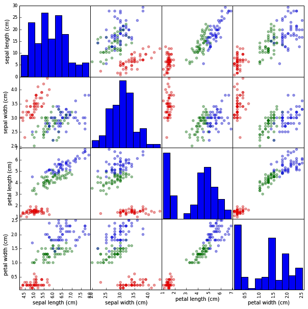
For example, let's just observe how classes can be easily separated when you wish to combine at least two of the four available variables by using a scatterplot matrix.

Scatterplot matrices are arranged in a matrix format, whose columns and rows are the dataset variables. The elements of the matrix contain single scatterplots whose x values are determined by the row variable of the matrix and y values by the column variable. The diagonal elements of the matrix may contain a distribution histogram or some other univariate representation of the variable at the same time in its row and column.

The pandas library offers an off-the-shelf function to quickly build scatterplot matrices and start exploring relationships and distributions between the quantitative variables in a dataset:

In: import pandas as pd
import numpy as np
colors = list()
palette = {0: "red", 1: "green", 2: "blue"}

In: for c in np.nditer(iris.target): colors.append(palette[int(c)])
# using the palette dictionary, we convert
# each numeric class into a color string
dataframe = pd.DataFrame(iris.data, columns=iris.feature_names)

In: sc = pd.scatter_matrix(dataframe, alpha=0.3, figsize=(10, 10),
diagonal='hist', color=colors, marker='o', grid=True)

The following is the output obtained after executing the preceding code:

We encourage you to experiment a lot with this dataset and with similar ones before you work on other complex real data because the advantage of focusing on an accessible, non-trivial data problem is that it can help you to quickly build your foundations on data science.

After a while anyway, though they are useful and interesting for your learning activities, toy datasets will start limiting the variety of different experimentations that you can achieve. In spite of the insights provided, in order to progress, you'll need to gain access to complex and realistic data science topics. Consequently, we will have to resort to some external data.

The MLdata.org and other public repositories for open source data

The second type of example dataset that we will present can be downloaded directly from the machine learning dataset repository, or from the LIBSVM data website. Contrary to the previous dataset, in this case, you will need access to the internet.

First, mldata.org is a public repository for machine learning datasets that is hosted by the TU Berlin University and supported by Pattern Analysis, Statistical Modelling, and Computational Learning (PASCAL), a network funded by the European Union. You are free to download any dataset from this repository and experiment with it.

For example, if you need to download all the data related to earthquakes since 1972, as reported by the United States Geological Survey, in order to analyze the data to search for predictive patterns, you will find the data repository at http://mldata.org/repository/data/viewslug/global-earthquakes/ (here, you will find a detailed description of the data).

Note that the directory that contains the dataset is global-earthquakes; you can directly obtain the data by using the following commands:

In: from sklearn.datasets import fetch_mldata
earthquakes = fetch_mldata('global-earthquakes')
print (earthquakes.data)
print (earthquakes.data.shape)

Out: (59209L, 4L)

As in the case of the Scikit-learn package toy dataset, the obtained object is a complex dictionary-like structure, where your predictive variables are earthquakes.data and your target to be predicted is earthquakes.target. This being the real data, in this case, you will have quite a lot of examples and just a few variables available.

LIBSVM data examples

LIBSVM Data (http://www.csie.ntu.edu.tw/~cjlin/libsvmtools/datasets/) is a page that gathers data from many other collections. It is maintained by Chih-Jen Lin, one of the authors of LIBSVM, a support vector machines learning algorithm for predictions (Chih-Chung Chang and Chih-Jen Lin, LIBSVM : a library for support vector machines. ACM Transactions on Intelligent Systems and Technology, 2:27:1--27:27, 2011). This offers different regression, binary, and multilabel classification datasets that are stored in the LIBSVM format. This repository is quite interesting if you wish to experiment with the support vector machine's algorithm, and, again, it is free for you to download and use the data.

If you want to load a dataset, first go to the web page where you can visualize the data on your browser. In the case of our example, visit http://www.csie.ntu.edu.tw/~cjlin/libsvmtools/datasets/binary/a1a and note down the address (a1a is a dataset that's originally from the UC Irvine Machine Learning Repository, another open source data repository). Then, you can proceed by performing a direct download using that address:

In: import urllib2
url =
'http://www.csie.ntu.edu.tw/~cjlin/libsvmtools/datasets/binary/a1a'
a2a = urllib2.urlopen(url)

In: from sklearn.datasets import load_svmlight_file
X_train, y_train = load_svmlight_file(a2a)
print (X_train.shape, y_train.shape)

Out: (1605, 119) (1605,)

In return, you will get two single objects: a set of training examples in a sparse matrix format and an array of responses.

Loading data directly from CSV or text files

Sometimes, you may have to download the datasets directly from their repository by using a web browser or a wget command (on Linux systems).

If you have already downloaded and unpacked the data (if necessary) into your working directory, the simplest way to load your data and start working is offered by the NumPy and the pandas library with their respective loadtxt and read_csv functions.

For instance, if you intend to analyze the Boston housing data and use the version present at http://mldata.org/repository/data/viewslug/regression-datasets-housing, you first have to download the regression-datasets-housing.csv file in your local directory.

You can use the following link for a direct download of the dataset: http://mldata.org/repository/data/download/csv/regression-datasets-housing.

Since the variables in the dataset are all numeric (13 continuous and one binary), the fastest way to load and start using it is by trying out the loadtxt NumPy function and directly loading all the data into an array.

Even in real-life datasets, you will often find mixed types of variables, which can be addressed by pandas.read_table or pandas.read_csv. Data can then be extracted by the values method; loadtxt can save a lot of memory if your data is already numeric. In fact, the loadtxt command doesn't require any in-memory duplication:

In: housing = np.loadtxt('regression-datasets-housing.csv', 
delimiter=',')
print (type(housing))

Out: <class 'numpy.ndarray'>

In: print (housing.shape)

Out: (506, 14)

The loadtxt function expects, by default, tabulation as a separator between the values on a file. If the separator is a colon (,) or a semicolon(;), you have to make it explicit by using the parameter delimiter:

>>>  import numpy as np
>>> type(np.loadtxt)
<type 'function'>
>>> help(np.loadtxt)
Help on the loadtxt function can be found in the numpy.lib.npyio module.

Another important default parameter is dtype, which is set to float.

This means that loadtxt will force all of the loaded data to be converted into a floating-point number.

If you need to determinate a different type (for example, int), you have to declare it beforehand.

For instance, if you want to convert numeric data to int, use the following code:

In: housing_int =housing.astype(int)

Printing the first three elements of the row of the housing and housing_int arrays can help you understand the difference:

In:  print (housing[0,:3], 'n', housing_int[0,:3])

Out: [ 6.32000000e-03 1.80000000e+01 2.31000000e+00]
[ 0 18 2]

Frequently, though not always the case in our example, the data on files feature in the first line of a textual header contains the name of the variables. In this situation, the parameter that is skipped will point out the row in the loadtxt file from where it will start reading the data. Being the header on row 0 (in Python, counting always starts from 0), the skip=1 parameter will save the day and allow you to avoid an error and fail to load your data.

The situation would be slightly different if you were to download the Iris dataset, which is present at http://mldata.org/repository/data/viewslug/datasets-uci-iris/. In fact, this dataset presents a qualitative target variable, class, which is a string that expresses the iris species. Specifically, it's a categorical variable with four levels.

Therefore, if you were to use the loadtxt function, you will get a value error because an array must have all its elements of the same type. The variable class is a string, whereas the other variables are constituted by floating-point values.

The pandas library offers the solution to this and many similar cases, thanks to its DataFrame data structure that can easily handle datasets in a matrix form (row per columns) that is made up of different types of variables.

First, just download the datasets-uci-iris.csv file and have it saved in your local directory.

The dataset can be downloaded from http://archive.ics.uci.edu/ml/machine-learning-databases/iris/. This archive is the UC Irvine Machine Learning Repository, which currently maintains 440 datasets as a service to the machine learning community. Apart from this Iris dataset, you are free to download and try any other dataset present in the repository.

At this point, using read_csv from pandas is quite straightforward:

In: iris_filename = 'datasets-uci-iris.csv'
iris = pd.read_csv(iris_filename, sep=',', decimal='.',
header=None, names= ['sepal_length', 'sepal_width', \
'petal_length', 'petal_width', 'target'])
print (type(iris))

Out: <class 'pandas.core.frame.DataFrame'>

In order to not make the snippets of code printed in this book too cumbersome, we often wrap it and make it nicely formatted. When necessary, in order to safely interrupt the code and wrap it to a new line, we use the backslash symbol \ as in the preceding code example. When rendering the code of the book by yourself, you can ignore backslash symbols and go on writing all of the instructions on the same line, or you can digit the backslash and start a new line continuing with the code instructions. Please be warned that typing the backslash and then continuing the instruction on the same line will cause an execution error.

Apart from the filename, you can specify the separator (sep), the way the decimal points are expressed (decimal), whether there is a header (in this case, header=None; normally, if you have a header, then header=0), and the name of the variable where there is one (you can use a list; otherwise, pandas will provide some automatic naming).

Also, we have defined names that use single words (instead of spaces, we used underscores). Thus, we can later directly extract single variables by calling them as we do for methods; for instance, iris.sepal_length will extract the sepal length data.

At this point, if you need to convert the pandas DataFrame into a couple of NumPy arrays that contain the data and target values, this can be done easily in a couple of commands:

In: iris_data = iris.values[:,:4]
iris_target, iris_target_labels = pd.factorize(iris.target)
print (iris_data.shape, iris_target.shape)

Out: (150, 4) (150,)

Scikit-learn sample generators

As a last learning resource, the Scikit-learn package also offers the possibility to quickly create synthetic datasets for regression, binary and multilabel classification, cluster analysis, and dimensionality reduction.

The main advantage of recurring synthetic data lies in its instantaneous creation in the working memory of your Python console. It is, therefore, possible to create bigger data examples without having to engage in long downloading sessions from the internet (and saving a lot of stuff on your disk).

For example, you may need to work on a classification problem involving a million data points:

In: from sklearn import datasets
X,y = datasets.make_classification(n_samples=10**6,
n_features=10, random_state=101)
print (X.shape, y.shape)

Out: (1000000, 10) (1000000,)

After importing just the datasets module, we ask, using the make_classification command, for one million examples (the n_samples parameter) and 10 useful features (n_features). The random_state should be 101, so we are assured that we can replicate the same datasets at a different time and in a different machine.

For instance, you can type the following command:

In: datasets.make_classification(1, n_features=4, random_state=101)

This will always give you the following output:

Out: (array([[-3.31994186, -2.39469384, -2.35882002,  1.40145585]]), 
array([0]))

No matter what the computer and the specific situation are, random_state assures deterministic results that make your experimentations perfectly replicable.

Defining the random_state parameter using a specific integer number (in this case, it's 101, but it may be any number that you prefer or find useful) allows easy replication of the same dataset on your machine, the way it is set up, on different operating systems, and on different machines.

By the way, did it take too long?

On a i3-2330M CPU @ 2.20 GHz machine, it takes this:

In: %timeit X,y = datasets.make_classification(n_samples=10**6, 
n_features=10, random_state=101)

Out: 1 loops, best of 3: 1.17 s per loop

If it doesn't seem like it did take too long on your machine, and if you are ready, having set up and tested everything up to this point, we can start our data science journey.

lock icon The rest of the chapter is locked
Register for a free Packt account to unlock a world of extra content!
A free Packt account unlocks extra newsletters, articles, discounted offers, and much more. Start advancing your knowledge today.
Unlock this book and the full library FREE for 7 days
Get unlimited access to 7000+ expert-authored eBooks and videos courses covering every tech area you can think of
Renews at $19.99/month. Cancel anytime
Banner background image