Chapter 4: Introduction to neuralnet and Evaluation Methods
Activity 15: Training a Neural Network
Solution:
- Attach the packages:
# Attach the packages
library(caret)
library(groupdata2)
library(neuralnet)
library(NeuralNetTools)
- Set the seed value for reproducibility and easier comparison:
# Set seed for reproducibility and easier comparison
set.seed(1)
- Load the GermanCredit dataset:
# Load the German Credit dataset
GermanCredit <- read.csv("GermanCredit.csv")
- Remove the Age column:
# Remove the Age column
GermanCredit$Age <- NULL
- Create balanced partitions such that all three partitions have the same ratio of each class:
# Partition with same ratio of each class in all three partitions
partitions <- partition(GermanCredit, p = c(0.6, 0.2),
cat_col = "Class")
train_set <- partitions[[1]]
dev_set <- partitions[[2]]
valid_set <- partitions[[3]]
- Find the preprocessing parameters for scaling and centering from the training set:
# Find scaling and centering parameters
params <- preProcess(train_set[, 1:6], method=c("center", "scale"))
- Apply standardization to the first six predictors in all three partitions, using the preProcess parameters from the previous step:
# Transform the training set
train_set[, 1:6] <- predict(params, train_set[, 1:6])
# Transform the development set
dev_set[, 1:6] <- predict(params, dev_set[, 1:6])
# Transform the validation set
valid_set[, 1:6] <- predict(params, valid_set[, 1:6])
- Train the neural network classifier:
# Train the neural network classifier
nn <- neuralnet(Class == "Good" ~ InstallmentRatePercentage +
ResidenceDuration + NumberExistingCredits,
train_set, linear.output = FALSE)
- Plot the network with its weights:
# Plot the network
plotnet(nn, var_labs=FALSE)
The output is as follows:

Figure 4.18: Neural network architecture using three predictors
- Print the error:
train_error <- nn$result.matrix[1]
train_error
The output is as follows:
## [1] 62.15447
The random initialization of the neural network weights can lead to slightly different results from one training to another. To avoid this, we use the set.seed() function at the beginning of the script, which helps when comparing models. We could also train the same model architecture with five different seeds to get a better sense of its performance.
Activity 16: Training and Comparing Neural Network Architectures
Solution:
- Attach the packages:
# Attach the packages
library(groupdata2)
library(caret)
library(neuralnet)
library(mlbench)
- Set the random seed to 1:
# Set seed for reproducibility and easier comparison
set.seed(1)
- Load the PimaIndiansDiabetes2 dataset:
# Load the PimaIndiansDiabetes2 dataset
PimaIndiansDiabetes2 <- read.csv("PimaIndiansDiabetes2.csv")
- Summarize the dataset.
summary(PimaIndiansDiabetes2)
The summary is as follows:
## pregnant glucose pressure triceps
## Min. : 0.000 Min. : 44.0 Min. : 24.00 Min. : 7.00
## 1st Qu.: 1.000 1st Qu.: 99.0 1st Qu.: 64.00 1st Qu.:22.00
## Median : 3.000 Median :117.0 Median : 72.00 Median :29.00
## Mean : 3.845 Mean :121.7 Mean : 72.41 Mean :29.15
## 3rd Qu.: 6.000 3rd Qu.:141.0 3rd Qu.: 80.00 3rd Qu.:36.00
## Max. :17.000 Max. :199.0 Max. :122.00 Max. :99.00
## NA's :5 NA's :35 NA's :227
##
## insulin mass pedigree age
## Min. : 14.00 Min. :18.20 Min. :0.0780 Min. :21.00
## 1st Qu.: 76.25 1st Qu.:27.50 1st Qu.:0.2437 1st Qu.:24.00
## Median :125.00 Median :32.30 Median :0.3725 Median :29.00
## Mean :155.55 Mean :32.46 Mean :0.4719 Mean :33.24
## 3rd Qu.:190.00 3rd Qu.:36.60 3rd Qu.:0.6262 3rd Qu.:41.00
## Max. :846.00 Max. :67.10 Max. :2.4200 Max. :81.00
## NA's :374 NA's :11
##
## diabetes
## neg:500
## pos:268
- Handle missing data (quick solution). Start by assigning the dataset to a new name:
# Assign/copy dataset to a new name
diabetes_data <- PimaIndiansDiabetes2
- Remove the triceps and insulin columns:
# Remove the triceps and insulin columns
diabetes_data$triceps <- NULL
diabetes_data$insulin <- NULL
- Remove all rows containing missing data (NAs):
# Remove all rows with NAs (missing data)
diabetes_data <- na.omit(diabetes_data)
- Partition the dataset into a training set (60%), a development set (20%), and a validation set (20%). Use cat_col="diabetes" to balance the ratios of each class between the partitions:
# Partition with same ratio of each class in all three partitions
partitions <- partition(diabetes_data, p = c(0.6, 0.2),
cat_col = "diabetes")
train_set <- partitions[[1]]
dev_set <- partitions[[2]]
valid_set <- partitions[[3]]
- Find the preProcess parameters for scaling and centering the first six features:
# Find scaling and centering parameters
params <- preProcess(train_set[, 1:6], method = c("center", "scale"))
- Apply the scaling and centering to each partition:
# Transform the training set
train_set[, 1:6] <- predict(params, train_set[, 1:6])
# Transform the development set
dev_set[, 1:6] <- predict(params, dev_set[, 1:6])
# Transform the validation set
valid_set[, 1:6] <- predict(params, valid_set[, 1:6])
- Train multiple neural network architectures. Adjust them by changing the number of nodes and/or layers. In the model formula, use diabetes == "pos":
# Training multiple neural nets
nn4 <- neuralnet(diabetes == "pos" ~ ., train_set,
linear.output = FALSE, hidden = c(3))
nn5 <- neuralnet(diabetes == "pos" ~ ., train_set,
linear.output = FALSE, hidden = c(2,1))
nn6 <- neuralnet(diabetes == "pos" ~ ., train_set,
linear.output = FALSE, hidden = c(3,2))
- Put the model objects into a list:
# Put the model objects into a list
models <- list("nn4"=nn4,"nn5"=nn5,"nn6"=nn6)
- Create one-hot encoding of the diabetes variable:
# Evaluating each model on the dev_set
# Create one-hot encoding of diabetes variable
dev_true_labels <- ifelse(dev_set$diabetes == "pos", 1, 0)
- Create a for loop for evaluating the models. By running the evaluations in a for loop, we avoid repeating the code:
# Evaluate one model at a time in a loop, to avoid repeating the code
for (i in 1:length(models)){
# Predict the classes in the development set
dev_predicted_probabilities <- predict(models[[i]], dev_set)
dev_predictions <- ifelse(dev_predicted_probabilities > 0.5, 1, 0)
# Create confusion Matrix
confusion_matrix <- confusionMatrix(as.factor(dev_predictions),
as.factor(dev_true_labels),
mode="prec_recall",
positive = "1")
# Print the results for this model
# Note: paste0() concatenates the strings
# to (name of model + " on the dev...")
print( paste0( names(models)[[i]], " on the development set: "))
print(confusion_matrix)
}
The output is as follows:
## [1] "nn4 on the development set: "
## Confusion Matrix and Statistics
##
## Reference
## Prediction 0 1
## 0 79 19
## 1 16 30
##
## Accuracy : 0.7569
## 95% CI : (0.6785, 0.8245)
## No Information Rate : 0.6597
## P-Value [Acc > NIR] : 0.007584
##
## Kappa : 0.4505
## Mcnemar's Test P-Value : 0.735317
##
## Precision : 0.6522
## Recall : 0.6122
## F1 : 0.6316
## Prevalence : 0.3403
## Detection Rate : 0.2083
## Detection Prevalence : 0.3194
## Balanced Accuracy : 0.7219
##
## 'Positive' Class : 1
##
## [1] "nn5 on the development set: "
## Confusion Matrix and Statistics
##
## Reference
## Prediction 0 1
## 0 77 16
## 1 18 33
##
## Accuracy : 0.7639
## 95% CI : (0.686, 0.8306)
## No Information Rate : 0.6597
## P-Value [Acc > NIR] : 0.004457
##
## Kappa : 0.4793
## Mcnemar's Test P-Value : 0.863832
##
## Precision : 0.6471
## Recall : 0.6735
## F1 : 0.6600
## Prevalence : 0.3403
## Detection Rate : 0.2292
## Detection Prevalence : 0.3542
## Balanced Accuracy : 0.7420
##
## 'Positive' Class : 1
##
## [1] "nn6 on the development set: "
## Confusion Matrix and Statistics
##
## Reference
## Prediction 0 1
## 0 76 14
## 1 19 35
##
## Accuracy : 0.7708
## 95% CI : (0.6935, 0.8367)
## No Information Rate : 0.6597
## P-Value [Acc > NIR] : 0.002528
##
## Kappa : 0.5019
## Mcnemar's Test P-Value : 0.486234
##
## Precision : 0.6481
## Recall : 0.7143
## F1 : 0.6796
## Prevalence : 0.3403
## Detection Rate : 0.2431
## Detection Prevalence : 0.3750
## Balanced Accuracy : 0.7571
##
## 'Positive' Class : 1
- As the nn6 model has the highest accuracy and F1 score, it is the best model.
- Evaluate the best model on the validation set. Start by creating the one-hot encoding of the diabetes variable in the validation set:
# Create one-hot encoding of Class variable
valid_true_labels <- ifelse(valid_set$diabetes == "pos", 1, 0)
- Use the best model to predict the diabetes variable in the validation set:
# Predict the classes in the validation set
predicted_probabilities <- predict(nn6, valid_set)
predictions <- ifelse(predicted_probabilities > 0.5, 1, 0)
- Create a confusion matrix:
# Create confusion Matrix
confusion_matrix <- confusionMatrix(as.factor(predictions),
as.factor(valid_true_labels),
mode="prec_recall", positive = "1")
- Print the results:
# Print the results for this model
# Note that by separating two function calls by ";"
# we can have multiple calls per line
print("nn6 on the validation set:"); print(confusion_matrix)
The output is as follows:
## [1] "nn6 on the validation set:"
## Confusion Matrix and Statistics
##
## Reference
## Prediction 0 1
## 0 70 16
## 1 25 35
##
## Accuracy : 0.7192
## 95% CI : (0.6389, 0.7903)
## No Information Rate : 0.6507
## P-Value [Acc > NIR] : 0.04779
##
## Kappa : 0.4065
## Mcnemar's Test P-Value : 0.21152
##
## Precision : 0.5833
## Recall : 0.6863
## F1 : 0.6306
## Prevalence : 0.3493
## Detection Rate : 0.2397
## Detection Prevalence : 0.4110
## Balanced Accuracy : 0.7116
##
## 'Positive' Class : 1
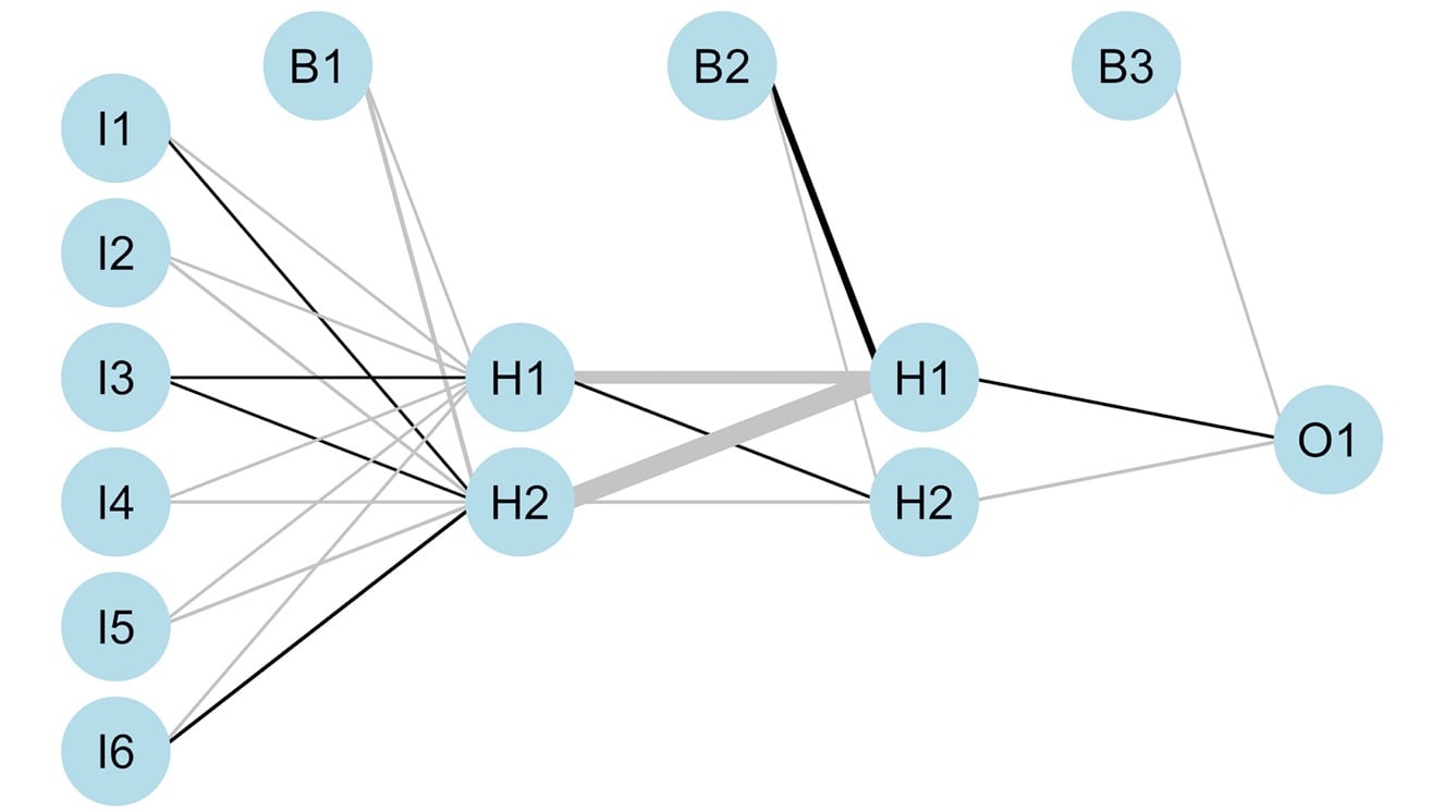
- Plot the best model:
plotnet(nn6, var_labs=FALSE)
The output will look as follows:

Figure 4.19: The best neural network architecture without cross-validation.
In this activity, we have trained multiple neural network architectures and evaluated the best model on the validation set.
Activity 17: Training and Comparing Neural Network Architectures with Cross-Validation
Solution:
- Attach the packages.
# Attach the packages
library(groupdata2)
library(caret)
library(neuralnet)
library(mlbench)
- Set the random seed to 1.
# Set seed for reproducibility and easier comparison
set.seed(1)
- Load the PimaIndiansDiabetes2 dataset.
# Load the PimaIndiansDiabetes2 dataset
data(PimaIndiansDiabetes2)
- Handle missing data (quick solution).
Start by assigning the dataset to a new name.
# Handling missing data (quick solution)
# Assign/copy dataset to a new name
diabetes_data <- PimaIndiansDiabetes2
- Remove the triceps and insulin columns.
# Remove the triceps and insulin columns
diabetes_data$triceps <- NULL
diabetes_data$insulin <- NULL
- Remove all rows with NAs.
# Remove all rows with Nas (missing data)
diabetes_data <- na.omit(diabetes_data)
- Partition the dataset into a training set (80%) and validation set (20%). Use cat_col="diabetes" to balance the ratios of each class between the partitions.
# Partition into a training set and a validation set
partitions <- partition(diabetes_data, p = 0.8, cat_col = "diabetes")
train_set <- partitions[[1]]
valid_set <- partitions[[2]]
- Find the preProcess parameters for scaling and centering the first six features.
# Find scaling and centering parameters
# Note: We could also decide to do this inside the training loop!
params <- preProcess(train_set[, 1:6], method=c("center", "scale"))
- Apply the scaling and centering to both partitions.
# Transform the training set
train_set[, 1:6] <- predict(params, train_set[, 1:6])
# Transform the validation set
valid_set[, 1:6] <- predict(params, valid_set[, 1:6])
- Create 4 folds in the training set, using the fold() function. Use cat_col="diabetes" to balance the ratios of each class between the folds.
# Create folds for cross-validation
# Balance on the Class variable
train_set <- fold(train_set, k=4, cat_col = "diabetes")
# Note: This creates a factor in the dataset called ".folds"
# Take care not to use this as a predictor.
- Write the cross-validation training section. Start by initializing the vectors for collecting errors and accuracies.
## Cross-validation loop
# Change the model formula in the loop and run the below
# for each model architecture you're testing
# Initialize vectors for collecting errors and accuracies
errors <- c()
accuracies <- c()
Start the training for loop. We have 4 folds, so we need 4 iterations.
# Training loop
for (part in 1:4){
- Assign the chosen fold as test set and the rest of the folds as train set. Be aware of the indentation.
# Assign the chosen fold as test set
# and the rest of the folds as train set
cv_test_set <- train_set[train_set$.folds == part,]
cv_train_set <- train_set[train_set$.folds != part,]
- Train the neural network with your chosen predictors.
# Train neural network classifier
# Make sure not to include the .folds column as a predictor!
nn <- neuralnet(diabetes == "pos" ~ .,
cv_train_set[, 1:7],
linear.output = FALSE,
hidden=c(2,2))
- Append the error to the errors vector.
# Append error to errors vector
errors <- append(errors, nn$result.matrix[1])
- Create one-hot encoding of the target variable in the CV test set.
# Create one-hot encoding of Class variable
true_labels <- ifelse(cv_test_set$diabetes == "pos", 1, 0)
- Use the trained neural network to predict the target variable in the CV test set.
# Predict the class in the test set
# It returns probabilities that the observations are "pos"
predicted_probabilities <- predict(nn, cv_test_set)
predictions <- ifelse(predicted_probabilities > 0.5, 1, 0)
- Calculate accuracy. We could also use confusionMatrix() here, if we wanted other metrics.
# Calculate accuracy manually
# Note: TRUE == 1, FALSE == 0
cv_accuracy <- sum(true_labels == predictions) / length(true_labels)
- Append the calculated accuracy to the accuracies vector.
# Append the accuracy to the accuracies vector
accuracies <- append(accuracies, cv_accuracy)
- Close the for loop.
}
- Calculate average_error and print it.
# Calculate average error and accuracy
# Note that we could also have gathered the predictions from all the
# folds and calculated the accuracy only once. This could lead to slightly
# different results, e.g. if the folds are not exactly the same size.
average_error <- mean(errors)
average_error
The output is as follows:
## [1] 28.38503
- Calculate average_accuracy and print it. Note that we could also have gathered the predictions from all the folds and calculated the accuracy only once.
average_accuracy <- mean(accuracies)
average_accuracy
The output is as follows:
## [1] 0.7529813
- Evaluate the best model architecture on the validation set. Start by training an instance of the model architecture on the entire training set.
# Once you have chosen the best model, train it on the entire training set
# and evaluate on the validation set
# Note that we set the stepmax, to make sure
# it has enough training steps to converge
nn_best <- neuralnet(diabetes == "pos" ~ .,
train_set[, 1:7],
linear.output = FALSE,
hidden=c(2,2),
stepmax = 2e+05)
- Create an one-hot encoding of the diabetes variable in the validation set.
# Find the true labels in the validation set
valid_true_labels <- ifelse(valid_set$diabetes == "pos", 1, 0)
- Use the model to predict the diabetes variable in the validation set.
# Predict the classes in the validation set
predicted_probabilities <- predict(nn_best, valid_set)
predictions <- ifelse(predicted_probabilities > 0.5, 1, 0)
- Create a confusion matrix.
# Create confusion matrix
confusion_matrix <- confusionMatrix(as.factor(predictions),
as.factor(valid_true_labels),
mode="prec_recall", positive = "1")
- Print the results.
# Print the results for this model
print("nn_best on the validation set:")
## [1] "nn_best on the validation set:"
print(confusion_matrix)
## Confusion Matrix and Statistics
##
## Reference
## Prediction 0 1
## 0 78 20
## 1 17 30
##
## Accuracy : 0.7448
## 95% CI : (0.6658, 0.8135)
## No Information Rate : 0.6552
## P-Value [Acc > NIR] : 0.01302
##
## Kappa : 0.4271
## Mcnemar's Test P-Value : 0.74231
##
## Precision : 0.6383
## Recall : 0.6000
## F1 : 0.6186
## Prevalence : 0.3448
## Detection Rate : 0.2069
## Detection Prevalence : 0.3241
## Balanced Accuracy : 0.7105
##
## 'Positive' Class : 1
##
- Plot the neural network.
plotnet(nn_best, var_labs=FALSE)
The output will be as follows:
