Advanced data transformation options
Now that you should be more comfortable working within the Power Query Editor, let's take the next step and discuss more advanced options. Often, you will find the need to go beyond these basic transforms when dealing with data that requires more care. In this section, you will learn about some common advanced transforms that you may have a need for, which include Conditional Columns, Fill Down, Unpivot, Merge Queries, and Append Queries.
Conditional Columns
Using the Power Query Editor Conditional Columns functionality is a great way to add new columns to your query that follow logical if/then/else statements. This concept of if/then/else is common across many programming languages, including Excel formulas. Let's review a real-world scenario where you would be required to do some data cleansing on a file before it could be used. In this example, you will be provided with a file of all the counties in the United States, and you must create a new column that extracts the state name from the county column and places it in its own column:
- Start by connecting to the
FIPS_CountyName.txtfile that is found in the book files using the Text/CSV connector. - Launch the Power Query Editor by selecting Transform Data, then start by changing the data type of
Column1to Text. When you do this, you will be prompted to replace an existing type conversion. You can accept this by clicking Replace current. - Now, on
Column2, filter out the value UNITED STATES from the column by clicking the arrow next to the column header and unchecking UNITED STATES. Then, click OK. - Remove the state abbreviation from
Column2by right-clicking on the column header and selecting Split Column | By Delimiter. Choose -- Custom -- for the delimiter type, and type , before then clicking OK, as shown in Figure 2.7:
Figure 2.7: Splitting a column based on a delimiter
- Next, rename the column names
Column1,Column 2.1, andColumn 2.2, toCounty Code,County Name, andState Abbreviation, respectively. - To isolate the full state name into its own column, you will need to implement Conditional Column. Go to the Add Column ribbon and select Conditional Column.
- Change the New column name property to
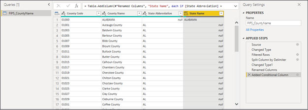
State Nameand implement the logicIf State Abbreviation equals null Then return County Name Else return nullas shown in Figure 2.8. To return the value from another column, you must select the icon in the Output property, then choose Select a column. Once this is complete, click OK:
Figure 2.8: Adding a conditional column
This results in a new column called State Name, which has the fully spelled-out state name only appearing on rows where the State Abbreviation is null:

Figure 2.9: End result of following these steps
This is only setting the stage to fully scrub this dataset. To complete the data cleansing process for this file, read on to the next section about Fill Down. However, for the purposes of this example, you have now learned how to leverage the capabilities of the Conditional Column transform in the Power Query Editor.
Fill Down
Fill Down is a rather unique transform in how it operates. By selecting Fill Down on a particular column, a value will replace all null values below it until another non-null appears. When another non-null value is present, that value will then fill down to all subsequent null values. To examine this transform, you will pick up from where you left off in the Conditional Column example in the previous section:
- Right-click on the State Name column header and select Transform | Capitalize Each Word. This transform should be self-explanatory.
- Next, select the State Name column and, in the Transform ribbon, select Fill | Down. This will take the value in the State Name column and replace all non-null values until there is another State Name value that it can switch to. After performing this transform, scroll through the results to ensure that the value of
Alabamaswitches toAlaskawhen appropriate. - To finish this example, filter out any
nullvalues that appear in the State Abbreviation column. The final result should look like Figure 2.10, as follows:
Figure 2.10: End result of following these steps
In this example, you learned how you can use Fill Down to replace all of the null values below a non-null value. You can also use Fill Up to do the opposite, which would replace all the null values above a non-null value. One important thing to note is that the data must be sorted properly for Fill Down or Fill Up to be successful. In the next section, you will learn about another advanced transform, known as Unpivot.
Unpivot
The Unpivot transform is an incredibly powerful transform that allows you to reorganize your dataset into a more structured format best suited for BI. Let's discuss this by visualizing a practical example to help understand the purpose of Unpivot. Imagine you are provided with a file that contains the populations of US states over the last three years, and looks as in Figure 2.11:

Figure 2.11: Example data that will cause problems in Power BI
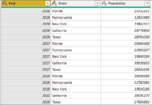
The problem with data stored like this is you cannot very easily answer simple questions. For example, how would you answer questions like, What was the total population for all states in the US in 2018? or What was the average state population in 2016? With the data stored in this format, simple reports are made rather difficult to design. This is where the Unpivot transform can be a lifesaver. Using Unpivot, you can change this dataset into something more acceptable for an analytics project, as shown in Figure 2.12:

Figure 2.12: Results of unpivoted data
Data stored in this format can now easily answer the questions posed earlier by simply dragging a few columns into your visuals. To accomplish this in other programming languages would often require fairly complex logic, while the Power Query Editor does it in just a few clicks.
There are three different methods for selecting the Unpivot transform that you should be aware of, and they include the following options:
- Unpivot Columns: Turns any selected columns, headers into row values and the data in those columns into a corresponding row. With this selection, any new columns that may get added to the data source will automatically be included in the Unpivot transform.
- Unpivot Other Columns: Turns all column headers that are not selected into row values and the data in those columns into a corresponding row. With this selection, any new columns that may get added to the data source will automatically be included in the Unpivot transform.
- Unpivot Only Selected Columns: Turns any selected columns' headers into row values and the data in those columns into a corresponding row. With this selection, any new columns that may get added to the data source will not be included in the Unpivot transform.
Let's walk through two examples of using the Unpivot transform to show you the first two of these methods, and provide an understanding of how this complex problem can be solved with little effort in Power BI. The third method mentioned for doing Unpivot will not be shown since it's so similar to the first option:
- Launch a new instance of the Power BI Desktop, and use the Excel connector to import the workbook called
Income Per Person.xlsxfound in the book source files. Once you select this workbook, choose the spreadsheet called Data in the Navigator window, and then select Transform Data to launch the Power Query Editor. Figure 2.13 shows what our data looks like before the Unpivot operation:
Figure 2.13: Example before Unpivot is performed
- Now, make the first row of data into column headers by selecting the transform called Use First Row as Headers on the Home ribbon.
- Rename the GDP per capita PPP, with projections column to Country.
- If you look closely at the column headers, you can tell that most of the column names are actually years and the values inside those columns are the income for those years. This is not the ideal way to store this data because it would be incredibly difficult to answer a question like, What is the average income per person for Belgium? To make it easier to answer this type of question, right-click on the Country column and select Unpivot Other Columns.
- Rename the columns
AttributeandValuetoYearandIncome, respectively. - To finish this first example, you should also rename this query Income. The results of these first steps can be seen in Figure 2.14:

Figure 2.14: Results of unpivoted data
This first method walked you through what can often be the fastest method for performing an Unpivot transform, which is by using the Unpivot Other Columns option. In this next example, you will learn how to use the Unpivot Columns method as well:
- Remain in the Power Query Editor, and select New Source from the Home ribbon. Use the Excel connector to import the
Total Population.xlsxworkbook from the book source files. Once you select this workbook, choose the spreadsheet called Data in the Navigator window, and then select OK. Figure 2.15 shows the dataset before Unpivot has been added:
Figure 2.15: Example before Unpivot is performed
- Like the last example, you will again need to make the first row of data into column headers by selecting the transform called Use First Row as Headers on the Home ribbon.
- Then, rename the column Total population to Country.
- This time, multi-select all the columns except Country, then right-click on one of the selected columns and choose Unpivot Other Columns as shown in Figure 2.16. The easiest way to multi-select these columns is to select the first column then hold Shift before clicking the last column:

Figure 2.16: Using the Unpivot Other Columns transform
- Rename the columns from Attribute and Value to Year and Population, respectively, to see the result showing in Figure 2.17:

Figure 2.17: Shows the final result of these steps
In this section, you learned about two different methods for performing an Unpivot. To complete the data cleansing process on these two datasets, it's recommended that you continue through the next section on merging queries.
Merge Query
Another common requirement when building BI solutions is the need to join two tables together to form a new outcome that includes some columns from both tables in the result. Fortunately, Power BI makes this task very simple with the Merge Queries feature. Using this feature requires that you select two tables and then determine which column or columns will be the basis of how the two queries are merged. After determining the appropriate columns for your join, you will select a join type. The join types are listed here with the description that is provided within the product:
- Left Outer (all rows from the first table, only matching rows from the second)
- Right Outer (all rows from the second table, only matching rows from the first)
- Full Outer (all rows from both tables)
- Inner (only matching rows from both tables)
- Left Anti (rows only in the first table)
- Right Anti (rows only in the second table)
Many of you may already be very familiar with these different join terms from SQL programming you have learned in the past. However, if these terms are new to you, I recommend reviewing Visualizing Merge Join Types in Power BI, courtesy of Jason Thomas in the Power BI Data Story Gallery: https://community.powerbi.com/t5/Data-Stories-Gallery/Visualizing-Merge-Join-Types-in-Power-BI/m-p/219906. This visual aid is a favorite of many users that are new to these concepts.
To examine the Merge Queries option, you will pick up from where you left off with the Unpivot examples in the previous section:
- With the Population query selected, find and select Merge Queries | Merge Queries as New on the Home ribbon.
- In the Merge dialog box, select the Income query from the drop-down selection in the middle of the screen.
- Then, multi-select the Country and Year columns on the Population query, and do the same under the Income query. This defines which columns will be used to join the two queries together. Ensure that the number indicators next to the column headers match, as demonstrated in Figure 2.18. If they don't, you could accidentally attempt to join on the incorrect columns.
- Next, select Inner (only matching rows) for Join Kind. This join type will return rows only when the columns you chose to join on have values that exist in both queries. Before you click OK, confirm that your screen matches Figure 2.18:

Figure 2.18: Configuring a merge between two queries
- Once you select OK, this will create a new query called
Merge1that combines the results of the two queries. Go ahead and rename this queryCountry Stats. - You will also notice that there is a column called
Incomethat has a value ofTablefor each row. This column is actually representative of the entireIncomequery that you joined to. To choose which columns you want from this query, click the Expand button on the column header. After clicking the Expand button, uncheck Country, Year, and Use original column name as prefix, then click OK. - Rename the column called
Income.1toIncome. Figure 2.19 shows this step completed:
Figure 2.19: Configuring a merge between two queries
- Finally, since you chose the option Merge Queries as New in Step 1, you can disable the load option for the original queries that you started with. To do this, right-click on the Income query in the Queries pane and click Enable load to disable it. Do the same thing for the Population query as shown in Figure 2.20. Disabling these queries means that the only query that will be loaded into your Power BI data model is the new one, called Country Stats:

Figure 2.20: Uncheck to disable the loading of this query into the data model
To begin using this dataset in a report, you would click Close & Apply. You will learn more about building reports in Chapter 5, Visualizing Data.
By default, merging queries together relies on exact matching values between your join column(s). However, you may work with data that does not always provide perfect matching values. For example, a user enters data and misspells their country as "Unite States" instead of United States. In those cases, you may consider the more advanced feature called Fuzzy Matching. With Fuzzy Matching, Power BI can perform an approximate match and still join on these two values based on the similarity of the values. In this section, you learned how the Merge Queries option is ideal for joining two queries together. In the next section, you will learn how you could solve the problem of performing a union of two or more queries.
Append Query
Occasionally, you will work with multiple datasets that need to be appended to each other. Here's a scenario: you work for a customer service department for a company that provides credit or loans to customers. You are regularly provided with .csv and .xlsx files that give summaries of customer complaints regarding credit cards and student loans. You would like to analyze both of these data extracts at the same time but, unfortunately, the credit card and student loan complaints are provided in two separate files. In this example, you will learn how to solve this problem by performing an append operation on these two different files:
- Launch a new instance of the Power BI Desktop, and use the Excel connector to import the workbook called
Student Loan Complaints.xlsxfound in the book source files. Once you select this workbook, choose the spreadsheet called Student Loan Complaints in the Navigator window, and then select Transform Data to launch the Power Query Editor. - Next, import the credit card data by selecting New Source | Text/CSV, then choose the file called
Credit Card Complaints.csvfound in the book source files. Click OK to bring this data into the Power Query Editor. - With the
Credit Card Complaintsquery selected, find and select Append Queries | Append Queries as New on the Home ribbon. - Select Student Loan Complaints as the table to append to, then select OK as shown in Figure 2.21:

Figure 2.21: Configuring an append between two queries
- Rename the newly created query All Complaints and view the results as seen in Figure 2.22:

Figure 2.22: Configuring an append between two queries
- Similar to the previous example, you would likely want to disable the load option for the original queries that you started with. To do this, right-click on the Student Load Complaints query in the Queries pane and click Enable load to disable it.
- Do the same to the Credit Card Complaints query, and then select Close & Apply.
Now that you have learned about the various methods for combining data, the next section will discuss a more advanced method of working with data using the R programming language.


