Search icon CANCEL
Subscription
0
Cart icon
Your Cart (0 item)
Close icon
You have no products in your basket yet
Save more on your purchases! discount-offer-chevron-icon
Savings automatically calculated. No voucher code required.
Arrow left icon
Explore Products
Best Sellers
New Releases
Books
Videos
Audiobooks
Learning Hub
Newsletter Hub
Free Learning
Arrow right icon
timer SALE ENDS IN
0 Days
:
00 Hours
:
00 Minutes
:
00 Seconds
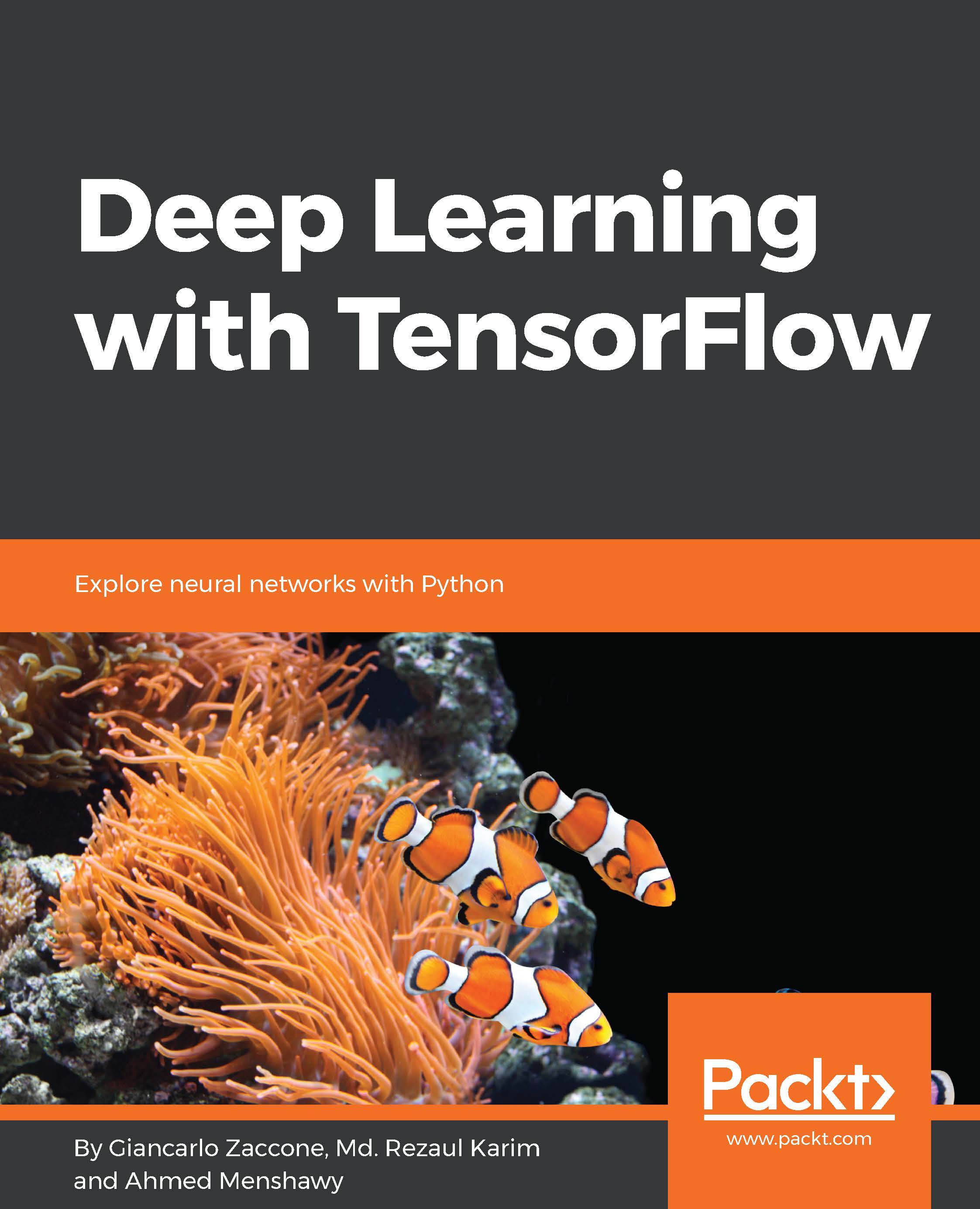
Deep Learning with TensorFlow

Deep Learning with TensorFlow: Explore neural networks with Python

Arrow left icon
Profile Icon Zaccone Profile Icon Milo Profile Icon Karim Profile Icon Menshawy
Arrow right icon
₱2806.99
Full star icon Full star icon Empty star icon Empty star icon Empty star icon 2 (10 Ratings)
Paperback Apr 2017 320 pages 1st Edition
eBook
₱579.99 ₱2245.99
Paperback
₱2806.99
Subscription
Free Trial
eBook
₱579.99 ₱2245.99
Paperback
₱2806.99
Subscription
Free Trial

What do you get with Print?

Product feature icon Instant access to your digital eBook copy whilst your Print order is Shipped
Product feature icon Paperback book shipped to your preferred address
Product feature icon Download this book in EPUB and PDF formats
Product feature icon Access this title in our online reader with advanced features
Product feature icon DRM FREE - Read whenever, wherever and however you want
OR
Modal Close icon
Payment Processing...
tick Completed

Shipping Address

Billing Address

Shipping Methods
Table of content icon View table of contents Preview book icon Preview Book

Deep Learning with TensorFlow

Getting Started with Deep Learning

In this chapter, we will discuss about some basic concepts of deep learning and their related architectures that will be found in all the subsequent chapters of this book. We'll start with a brief definition of machine learning, whose techniques allow the analysis of large amounts of data to automatically extract information and to make predictions about subsequent new data. Then we'll move onto deep learning, which is a branch of machine learning based on a set of algorithms that attempt to model high-level abstractions in data.

Finally, we'll introduce deep learning architectures, the so-called Deep Neural Networks (DNNs)--these are distinguished from the more commonplace single hidden layer neural networks by their depth; that is, the number of node layers through which data passes in a multistep process of pattern recognition. we will provide a chart summarizing all the neural networks from where most of the deep learning algorithm evolved.

In the final part of the chapter, we'll briefly examine and compare some deep learning frameworks across various features, such as the native language of the framework, multi-GPU support, and aspects of usability.

This chapter covers the following topics:

  • Introducing machine learning
  • What is deep learning?
  • Neural networks
  • How does an artificial neural network learn?
  • Neural network architectures
  • DNNs architectures
  • Deep learning framework comparison

Introducing machine learning

Machine learning is a computer science research area that deals with methods to identify and implement systems and algorithms by which a computer can learn, based on the examples given in the input. The challenge of machine learning is to allow a computer to learn how to automatically recognize complex patterns and make decisions that are as smart as possible. The entire learning process requires a dataset as follows:

  • Training set: This is the knowledge base used to train the machine learning algorithm. During this phase, the parameters of the machine learning model (hyperparameters) can be tuned according to the performance obtained.
  • Testing set: This is used only for evaluating the performance of the model on unseen data.

Learning theory uses mathematical tools that are derived from probability theory of and information theory. This allows you to assess the optimality of some methods over others.

There are basically three learning paradigms that will be briefly discussed:

  • Supervised learning
  • Unsupervised learning
  • Learning with reinforcement

Let's take a look at them.

Supervised learning

Supervised learning is the automatic learning task simpler and better known. It is based on a number of preclassified examples, in which, namely, is known a prior the category to which each of the inputs used as examples should belong. In this case, the crucial issue is the problem of generalization. After the analysis of a sample (often small) of examples, the system should produce a model that should work well for all possible inputs.

The set consists of labeled data, that is, objects and their associated classes. This set of labeled examples, therefore, constitutes the training set.

Most of the supervised learning algorithms share one characteristic: the training is performed by the minimization of a particular loss or cost function, representing the output error provided by the system with respect to the desired possible output, because the training set provides us with what must be the desired output.

The system then changes its internal editable parameters, the weights, to minimize this error function. The goodness of the model is evaluated, providing a second set of labeled examples (the test set), evaluating the percentage of correctly classified examples and the percentage of misclassified examples.

The supervised learning context includes the classifiers, but also the learning of functions that predict numeric values. This task is the regression. In a regression problem, the training set is a pair formed by an object and the associated numeric value. There are several supervised learning algorithms that have been developed for classification and regression. These can be grouped into the formula used to represent the classifier or the learned predictor, among all, decision trees, decision rules, neural networks and Bayesian networks.

Unsupervised learning

In unsupervised learning, a set of inputs is supplied to the system during the training phase which, however, contrary to the case supervised learning, is not labeled with the related belonging class. This type of learning is important because in the human brain it is probably far more common than supervised learning.

The only objects in the domain of learning models, in this case, are the observed data inputs, which often is assumed to be independent samples of an unknown underlying probability distribution.

Unsupervised learning algorithms are used particularly used in clustering problems, in which given a collection of objects, we want to be able to understand and show their relationships. A standard approach is to define a similarity measure between two objects, and then look for any cluster of objects that are more similar to each other, compared to the objects in the other clusters.

Reinforcement learning

Reinforcement learning is an artificial intelligence approach that emphasizes the learning of the system through its interactions with the environment. With reinforcement learning, the system adapts its parameters based on feedback received from the environment, which then provides feedback on the decisions made. For example, a system that models a chess player who uses the result of the preceding steps to improve their performance is a system that learns with reinforcement. Current research on learning with reinforcement is highly interdisciplinary, and includes researchers specializing in genetic algorithms, neural networks, psychology, and control engineering.

The following figure summarizes the three types of learning, with the related problems to address:

Figure 1: Types of learning and related problems

What is deep learning?

Deep learning is a machine learning research area that is based on a particular type of learning mechanism. It is characterized by the effort to create a learning model at several levels, in which the most profound levels take as input the outputs of previous levels, transforming them and always abstracting more. This insight on the levels of learning is inspired by the way the brain processes information and learns, responding to external stimuli.

Each learning level corresponds, hypothetically, to one of the different areas which make up the cerebral cortex.

How the human brain works

The visual cortex, which is intended to solve image recognition problems, shows a sequence of sectors placed in a hierarchy. Each of these areas receives an input representation, by means of flow signals that connect it to other sectors.

Each level of this hierarchy represents a different level of abstraction, with the most abstract features defined in terms of those of the lower level. At a time when the brain receives an input image, the processing goes through various phases, for example, detection of the edges or the perception of forms (from those primitive to those gradually more and more complex).

As the brain learns by trial and activates new neurons by learning from the experience, even in deep learning architectures, the extraction stages or layers are changed based on the information received at the input.

The scheme, on the next page shows what has been said in the case of an image classification system, each block gradually extracts the features of the input image, going on to process data already preprocessed from the previous blocks, extracting features of the image that are increasingly abstract, and thus building the hierarchical representation of data that comes with on deep learning based system.

More precisely, it builds the layers as follows along with the figure representation:

  • Layer 1: The system starts identifying the dark and light pixels
  • Layer 2: The system identifies edges and shapes
  • Layer 3: The system learns more complex shapes and objects
  • Layer 4: The system learns which objects define a human face

Here is the visual representation of the process:

Figure 2: A deep learning system at work on a facial classification problem

Deep learning history

The development of deep learning consequently occurred parallel to the study of artificial intelligence, and especially neural networks. After beginning in the 50 s, it is mainly in the 80s that this area grew, thanks to Geoff Hinton and machine learning specialists who collaborated with him. In those years, computer technology was not sufficiently advanced to allow a real improvement in this direction, so we had to wait until the present day to see, thanks to the availability of data and the computing power, even more significant developments.

Problems addressed

As for the areas of application, deep learning is employed in the development of speech recognition systems, in the search patterns, and especially, in the image recognition, thanks to its learning characteristics for levels, which enable it to focus, step by step, on the various areas of an image to be processed and classified.

Neural networks

Artificial Neural Networks (ANNs) are one of the main tools that take advantage of the concept of deep learning. They are an abstract representation of our nervous system, which contains a collection of neurons that communicate with each other through connections called axons. The first artificial neuron model was proposed in 1943 by McCulloch and Pitts in terms of a computational model of nervous activity. This model was followed by another, proposed by John von Neumann, Marvin Minsky, Frank Rosenblatt (the so-called perceptron), and many others.

The biological neuron

As you can see in the following figure, a biological neuron is composed of the following:

  • A cell body or soma
  • One or more dendrites, whose responsibility is to receive signals from other neurons
  • An axon, which in turn conveys the signals generated by the same neuron to the other connected neurons

This is what a biological neuron model looks like:

Figure 3: Biological neuron model

The neuron activity is in the alternation of sending the signal (active state) and rest/reception of signals from other neurons (inactive state).

The transition from one phase to another is caused by the external stimuli represented by signals that are picked up by the dendrites. Each signal has an excitatory or inhibitory effect, conceptually represented by a weight associated with the stimulus. The neuron in an idle state accumulates all the signals received until they have reached a certain activation threshold.

An artificial neuron

Similar to the biological one, the artificial neuron consists of the following:

  • One or more incoming connections, with the task of collecting numerical signals from other neurons; each connection is assigned a weight that will be used to consider each signal sent
  • One or more output connections that carry the signal for the other neurons
  • An activation function determines the numerical value of the output signal, on the basis of the signals received from the input connections with other neurons, and suitably collected from the weights associated with each picked-up signal and the activation threshold of the neuron itself

The following figure represents the artificial neuron:

Figure 4: Artificial neuron model

The output, that is, the signal whereby the neuron transmits its activity outside, is calculated by applying the activation function, also called the transfer function, to the weighted sum of the inputs. These functions have a dynamic between -1 and 1, or between 0 and 1.

There is a set of activation functions that differs in complexity and output:

  • Step function: This fixes the threshold value x (for example, x= 10). The function will return 0 or 1 if the mathematical sum of the inputs is at, above, or below the threshold value.
  • Linear combination: Instead of managing a threshold value, the weighted sum of the input values is subtracted from a default value; we will have a binary outcome, but it will be expressed by a positive (+b) or negative (-b) output of the subtraction.
  • Sigmoid: This produces a sigmoid curve, a curve having an S trend. Often, the sigmoid function refers to a special case of the logistic function.

From the simplest forms, used in the prototyping of the first artificial neurons, we then move on to more complex ones that allow greater characterization of the functioning of the neuron. The following are just a few:

  • Hyperbolic tangent function
  • Radial basis function
  • Conic section function
  • Softmax function

It should be recalled that the network, and then the weights in the activation functions, will then be trained. As the selection of the activation function is an important task in the implementation of the network architecture, studies indicate marginal differences in terms of output quality if the training phase is carried out properly.

Figure 5: Most used transfer functions

In the preceding figure, the functions are labeled as follows:

  • a: Step function
  • b: Linear function
  • c: Computed sigmoid function with values between 0 and 1
  • d: Sigmoid function with computed values between -1 and 1

How does an artificial neural network learn?

The learning process of a neural network is configured as an iterative process of optimization of the weights, and is therefore of the supervised type. The weights are modified based on the network performance on a set of examples belonging to the training set, where the category they belong to is known. The aim is to minimize a loss function, which indicates the degree to which the behavior of the network deviates from the desired one. The performance of the network is then verified on a test set consisting of objects (for example, images in a image classification problem) other than those of the training set.

The backpropagation algorithm

A supervised learning algorithm used is the backpropagation algorithm.

The basic steps of the training procedure are as follows:

  1. Initialize the net with random weights.
  2. For all training cases:
    • Forward pass: Calculates the error committed by the net, the difference between the desired output and the actual output.
    • Backward pass: For all layers, starting with the output layer, back to the input layer.
  3. Show the network layer output with correct input (error function).
  4. Adapt weights in the current layer to minimize the error function. This is the backpropagation's optimization step. The training process ends when the error on the validation set begins to increase, because this could mark the beginning of a phase of over-fitting of the network, that is, the phase in which the network tends to interpolate the training data at the expense of generalization ability.

Weights optimization

The availability of efficient algorithms to weights optimization, therefore, constitutes an essential tool for the construction of neural networks. The problem can be solved with an iterative numerical technique called gradient descent (GD).

This technique works according to the following algorithm:

  1. Some initial values for the parameters of the model are chosen randomly.
  2. Compute the gradient G of the error function with respect to each parameter of the model.
  3. Change the model's parameters so that they move in the direction of decreasing the error, that is, in the direction of -G.
  4. Repeat steps 2 and 3 until the value of G approaches zero.
In mathematics, the gradient of a scalar field is a real-valued function of several variables, then defined in a region of a space in two, three, or more dimensions. The gradient of a function is defined as the vector that has Cartesian components for the partial derivatives of the function. The gradient represents the direction of maximum increment of a function of n variables: f (x1, x2,...., xn). The gradient is then a vector quantity that indicates a physical quantity as a function of its various different parameters.

The gradient G of the error function E provides the direction in which the error function with the current values has the steeper slope, so to decrease E, we have to make some small steps in the opposite direction, -G (see the following figures).

By repeating this operation several times in an iterative manner, we move in the direction in which the gradient G of the function E is minimal (see the following figure):

Figure 6: Gradient descent procedure

As you can see, we move in the direction in which the gradient G of the function E is minimal.

Stochastic gradient descent

In GD optimization, we compute the cost gradient based on the complete training set; hence, we sometimes also call it batch GD. In the case of very large datasets, using GD can be quite costly, since we are only taking a single step for one pass over the training set. Thus, the larger the training set, the slower our algorithm updates the weights and the longer it may take until it converges to the global cost minimum.

An alternative approach and the fastest of gradient descent, and for this reason, used in DNNs, is the Stochastic Gradient Descent (SGD).

In SGD, we use only one training sample from the training set to do the update for a parameter in a particular iteration. Here, the term stochastic comes from the fact that the gradient based on a single training sample is a stochastic approximation of the true cost gradient.

Due to its stochastic nature, the path toward the global cost minimum is not direct, as in GD, but may zigzag if we are visualizing the cost surface in a 2D space (see the following figure, (b) Stochastic Gradient Descent - SDG).

We can make a comparison between these optimization procedures, showing the next figure, the gradient descent (see the following figure, (a) Gradient Descent - GD) assures that each update in the weights is done in the right direction--the one that minimizes the cost function. With the growth of datasets' size, and more complex computations in each step, SGD came to be preferred in these cases. Here, updates to the weights are done as each sample is processed and, as such, subsequent calculations already use improved weights. Nonetheless, this very reason leads to it incurring some misdirection in minimizing the error function:

Figure 7: GD versus SDG

Neural network architectures

The way to connect the nodes, the number of layers present, that is, the levels of nodes between input and output, and the number of neurons per layer, defines the architecture of a neural network. There are various types of architecture in neural networks, but this book will focus mainly on two large architectural families.

Multilayer perceptron

In multilayer networks, one can identify the artificial neurons of layers such that:

  • Each neuron is connected with all those of the next layer
  • There are no connections between neurons belonging to the same layer
  • There are no connections between neurons belonging to non-adjacent layers
  • The number of layers and of neurons per layer depends on the problem to be solved

The input and output layers define inputs and outputs; there are hidden layers, whose complexity realizes different behaviors of the network. Finally, the connections between neurons are represented by as many matrices are the pairs of adjacent layers. Each array contains the weights of the connections between the pairs of nodes of two adjacent layers. The feed-forward networks are networks with no loops within the layers.

Following is the graphical representation of multilayer perceptron architecture:

Figure 8: A multilayer perceptron architecture

DNNs architectures

Deep Neural Networks (DNNs) are artificial neural networks strongly oriented to deep learning. Where normal procedures of analysis are inapplicable due to the complexity of the data to be processed, such networks are an excellent modeling tool. DNNs are neural networks, very similar to those we have discussed, but they must implement a more complex model (a great number of neurons, hidden layers, and connections), although they follow the learning principles that apply to all machine learning problems (that is, supervised learning).

As they are built, the DNNs work in parallel, so they are able to treat a lot of data. They are a sophisticated statistical system, equipped with a good immunity to errors.

Unlike algorithmic systems where you can examine the output generation step by step, in neural networks, you can also have very reliable results, but sometimes without the ability to understand the reasons for those results. There are no theorems to generate optimal neural networks--the likelihood of getting a good network is all in the hands of its creator, who must be familiar with statistical concepts, and particular attention must be given to the choice of predictor variables.

For brief cheat sheet on the different neural network architecture and their related publications, refer to the website of Asimov Institute at http://www.asimovinstitute.org/neural-network-zoo/.

Finally, we observe that, in order to be productive, the DNNs require training that properly tunes the weights. Training can take a long time if the data to be examined and the variables involved are high, as is often the case when you want optimal results. This section introduces the deep learning architectures that we will cover during the course of this book.

Convolutional Neural Networks

Convolutional Neural Networks (CNNs) has been designed specifically for image recognition. Each image used in learning is divided into compact topological portions, each of which will be processed by filters to search for particular patterns. Formally, each image is represented as a three-dimensional matrix of pixels (width, height, and color), and every sub-portion is put on convolution with the filter set. In other words, scrolling each filter along the image computes the inner product of the same filter and input. This procedure produces a set of feature maps (activation maps) for the various filters. By superimposing the various feature maps of the same portion of the image, we get an output volume. This type of layer is called a convolutional layer.

The following figure shows a typical CNN architecture:

Figure 9: Convolutional neural network architecture

Restricted Boltzmann Machines

A Restricted Boltzmann Machine (RBM) consists of a visible and a hidden layer of nodes, but without visible-visible connections and hidden-hidden by the term restricted. These restrictions allow more efficient network training (training that can be supervised or unsupervised).

This type of neural network can represent with few size of the network a large number of features of the inputs; in fact, the n hidden nodes can represent up to 2n features. The network can be trained to respond to a single question (yes/no), up until (again, in binary terms) a total of 2n questions.

The architecture of the RBM is as follows, with neurons arranged according to a symmetrical bipartite graph:

Figure 10: Restricted Boltzmann Machine architecture

Autoencoders

Stacked autoencoders are DNNs that are typically used for data compression. Their particular hourglass structure clearly shows the first part of the process, where the input data is compressed, up to the so-called bottleneck, from which the decompression starts.

The output is then an approximation of the input. These networks are not supervised in the pretraining (compression) phase, and the fine-tuning (decompression) phase is supervised:

Figure 11: Stack autoencoder architecture

Recurrent Neural Networks

The fundamental feature of a Recurrent Neural Network (RNN) is that the network contains at least one feedback connection, so the activations can flow around in a loop. It enables the networks to do temporal processing and learn sequences, for example, perform sequence recognition/reproduction or temporal association/prediction. RNN architectures can have many different forms. One common type consists of a standard multilayer perceptron (MLP) plus added loops. These can exploit the powerful non-linear mapping capabilities of the MLP, and also have some form of memory. Others have more uniform structures, potentially with every neuron connected to all the others, and may also have stochastic activation functions. For simple architectures and deterministic activation functions, learning can be achieved using similar gradient descent procedures to those leading to the backpropagation algorithm for feed-forward networks.

The following figure shows a few of the most important types and features of RNNs:

Figure 12: Recurrent Neural Network architecture

Deep learning framework comparisons

In this section, we will look at some of the most popular frameworks regarding deep learning. In short, almost all libraries provide the possibility of using the graphics processor to speed up the learning process, and are released under an open license and are the result of implementation by university research groups.Before starting the comparison, refer figure 13 which is one of the most complete charts of neural networks till date. If you see the URL and related papers, you will find that the idea of neural networks is pretty old and the software frameworks that we are going to compare below also adapts similar architecture during their framework development:


Figure 13: complete charts of neural networks (Source: http://www.asimovinstitute.org/neural-network-zoo/)

  • Theano: This is probably the most widespread library. Written in Python, one of the languages most used in the field of machine learning (also in TensorFlow), allows the calculation also GPU, coming to have 24x the performance of the CPU. It allows you to define, optimize, and evaluate complex mathematical expressions such as multidimensional arrays.
  • Caffe: This was developed primarily by Berkeley Vision and Learning Center (BVLC), and is a framework designed to stand out in terms of expression, speed, and modularity. Its unique architecture encourages application and innovation by allowing easier transition from calculation of CPU to GPU. The large community of users allowed for considerable development in recent times. It is written in Python, but the installation process can be long due to the numerous support libraries to compile.
  • Torch: This is a vast ecosystem for machine learning which offers a large number of algorithms and functions, including those for deep learning and processing of various types of multimedia, such as audio and video data, with particular attention to parallel computing. It provides an excellent interface for the C language and has a large community of users. Torch is a library that extends the scripting language Lua, and is intended to provide a flexible environment for designing and training machine learning systems. Torch is a self-contained and highly portable framework on each platform (for example, Windows, Mac, Linux, and Android) and scripts manage to run on these platforms without modification. The Torch package provides many useful features for different applications.

Finally, the following table provides a summary of each framework's salient features, including TensorFlow, which will be described (of course!!) in the coming chapters:

TensorFlow Torch Caffe Theano

Programming language

used

Python and C++ Lua C++ Python
GPU card support Yes Yes Yes By default, no
Pros
  • Computational graph abstraction, like Theano
  • Faster compile times than Theano
  • TensorBoard for visualization
  • Data and model parallelism
  • Easy to set up
  • Helpful error messages
  • Large amount of sample code and tutorials
  • Good for feedforward networks and image processing
  • Good for fine tuning existing networks
  • Python interface is pretty useful
  • Expressive Python syntax
  • Higher-level spin-off frameworks
  • Large amount of sample code and tutorials
Cons
  • Slower than other frameworks
  • Not many pre-trained models
  • Computational graph is pure Python, therefore slow
  • No commercial support
  • Can be somewhat difficult to set up in CentOS
  • Error messages are cryptic
  • Need to write C++ / CUDA for new GPU layers
  • Not good for recurrent networks
  • No commercial support
  • Error messages can be unhelpful
  • Large models can have long compile times
Deep learning framework comparison

Summary

In this chapter, we introduced some of the fundamental themes of deep learning. It consists of a set of methods that allow a machine learning system to obtain a hierarchical representation of data, on multiple levels. This is achieved by combining simple units, each of which transforms the representation at its own level, starting from the input level, in a representation at a higher level, slightly more abstract.

In recent years, these techniques have provided results never seen before in many applications, such as image recognition and speech recognition. One of the main reasons for the spread of these techniques has been the development of GPU architectures, which considerably reduced the training time of DNNs. There are different DNN architectures, each of which has been developed for a specific problem. We'll talk more about those architectures in later chapters, showing examples of applications created with the TensorFlow framework.

The chapter ended with a brief overview of the implemented deep learning frameworks.

In the next chapter, we begin our journey into deep learning, introducing the TensorFlow software library. We will describe its main features and look at how to install it and set up a first working session.

Left arrow icon Right arrow icon
Download code icon Download Code

Key benefits

  • Learn how to implement advanced techniques in deep learning with Google’s brainchild, TensorFlow
  • Explore deep neural networks and layers of data abstraction with the help of this comprehensive guide
  • Real-world contextualization through some deep learning problems concerning research and application

Description

Deep learning is the step that comes after machine learning, and has more advanced implementations. Machine learning is not just for academics anymore, but is becoming a mainstream practice through wide adoption, and deep learning has taken the front seat. As a data scientist, if you want to explore data abstraction layers, this book will be your guide. This book shows how this can be exploited in the real world with complex raw data using TensorFlow 1.x. Throughout the book, you’ll learn how to implement deep learning algorithms for machine learning systems and integrate them into your product offerings, including search, image recognition, and language processing. Additionally, you’ll learn how to analyze and improve the performance of deep learning models. This can be done by comparing algorithms against benchmarks, along with machine intelligence, to learn from the information and determine ideal behaviors within a specific context. After finishing the book, you will be familiar with machine learning techniques, in particular the use of TensorFlow for deep learning, and will be ready to apply your knowledge to research or commercial projects.

Who is this book for?

The book is intended for a general audience of people interested in machine learning and machine intelligence. A rudimentary level of programming in one language is assumed, as is a basic familiarity with computer science techniques and technologies, including a basic awareness of computer hardware and algorithms. Some competence in mathematics is needed to the level of elementary linear algebra and calculus.

What you will learn

  • Learn about machine learning landscapes along with the historical development and progress of deep learning
  • Learn about deep machine intelligence and GPU computing with the latest TensorFlow 1.x
  • Access public datasets and utilize them using TensorFlow to load, process, and transform data
  • Use TensorFlow on real-world datasets, including images, text, and more
  • Learn how to evaluate the performance of your deep learning models
  • Using deep learning for scalable object detection and mobile computing
  • Train machines quickly to learn from data by exploring reinforcement
  • learning techniques
  • Explore active areas of deep learning research and applications
Estimated delivery fee Deliver to Philippines

Standard delivery 10 - 13 business days

₱492.95

Premium delivery 5 - 8 business days

₱2548.95
(Includes tracking information)

Product Details

Country selected
Publication date, Length, Edition, Language, ISBN-13
Publication date : Apr 24, 2017
Length: 320 pages
Edition : 1st
Language : English
ISBN-13 : 9781786469786
Vendor :
Google
Category :
Languages :
Concepts :
Tools :

What do you get with Print?

Product feature icon Instant access to your digital eBook copy whilst your Print order is Shipped
Product feature icon Paperback book shipped to your preferred address
Product feature icon Download this book in EPUB and PDF formats
Product feature icon Access this title in our online reader with advanced features
Product feature icon DRM FREE - Read whenever, wherever and however you want
OR
Modal Close icon
Payment Processing...
tick Completed

Shipping Address

Billing Address

Shipping Methods
Estimated delivery fee Deliver to Philippines

Standard delivery 10 - 13 business days

₱492.95

Premium delivery 5 - 8 business days

₱2548.95
(Includes tracking information)

Product Details

Publication date : Apr 24, 2017
Length: 320 pages
Edition : 1st
Language : English
ISBN-13 : 9781786469786
Vendor :
Google
Category :
Languages :
Concepts :
Tools :

Packt Subscriptions

See our plans and pricing
Modal Close icon
$19.99 billed monthly
Feature tick icon Unlimited access to Packt's library of 7,000+ practical books and videos
Feature tick icon Constantly refreshed with 50+ new titles a month
Feature tick icon Exclusive Early access to books as they're written
Feature tick icon Solve problems while you work with advanced search and reference features
Feature tick icon Offline reading on the mobile app
Feature tick icon Simple pricing, no contract
$199.99 billed annually
Feature tick icon Unlimited access to Packt's library of 7,000+ practical books and videos
Feature tick icon Constantly refreshed with 50+ new titles a month
Feature tick icon Exclusive Early access to books as they're written
Feature tick icon Solve problems while you work with advanced search and reference features
Feature tick icon Offline reading on the mobile app
Feature tick icon Choose a DRM-free eBook or Video every month to keep
Feature tick icon PLUS own as many other DRM-free eBooks or Videos as you like for just ₱260 each
Feature tick icon Exclusive print discounts
$279.99 billed in 18 months
Feature tick icon Unlimited access to Packt's library of 7,000+ practical books and videos
Feature tick icon Constantly refreshed with 50+ new titles a month
Feature tick icon Exclusive Early access to books as they're written
Feature tick icon Solve problems while you work with advanced search and reference features
Feature tick icon Offline reading on the mobile app
Feature tick icon Choose a DRM-free eBook or Video every month to keep
Feature tick icon PLUS own as many other DRM-free eBooks or Videos as you like for just ₱260 each
Feature tick icon Exclusive print discounts

Frequently bought together


Stars icon
Total 8,726.97
TensorFlow Machine Learning Cookbook
₱3112.99
Deep Learning with TensorFlow
₱2806.99
Deep Learning with Keras
₱2806.99
Total 8,726.97 Stars icon
Banner background image

Table of Contents

10 Chapters
Getting Started with Deep Learning Chevron down icon Chevron up icon
First Look at TensorFlow Chevron down icon Chevron up icon
Using TensorFlow on a Feed-Forward Neural Network Chevron down icon Chevron up icon
TensorFlow on a Convolutional Neural Network Chevron down icon Chevron up icon
Optimizing TensorFlow Autoencoders Chevron down icon Chevron up icon
Recurrent Neural Networks Chevron down icon Chevron up icon
GPU Computing Chevron down icon Chevron up icon
Advanced TensorFlow Programming Chevron down icon Chevron up icon
Advanced Multimedia Programming with TensorFlow Chevron down icon Chevron up icon
Reinforcement Learning Chevron down icon Chevron up icon

Customer reviews

Top Reviews
Rating distribution
Full star icon Full star icon Empty star icon Empty star icon Empty star icon 2
(10 Ratings)
5 star 10%
4 star 10%
3 star 10%
2 star 10%
1 star 60%
Filter icon Filter
Top Reviews

Filter reviews by


Verified Amazon Customer Jul 22, 2017
Full star icon Full star icon Full star icon Full star icon Full star icon 5
Excellent book. It contains lots of practical examples. However, when I copied the codes from the book, there were some alignment issues and some codes were not executed correctly. Therefore, I had to manually fixed them.Fortunately, the authors have fixed all the minor bugs and the updated codes that I have downloaded from GitHub/Deep-Learning-with-TensorFlow are working perfectly.
Amazon Verified review Amazon
Ambuj Jan 07, 2018
Full star icon Full star icon Full star icon Full star icon Empty star icon 4
Good introduction if you want to start with tensor flow
Amazon Verified review Amazon
Matthew R. Versaggi Jan 03, 2018
Full star icon Full star icon Full star icon Empty star icon Empty star icon 3
I had such high hopes for this book - the theory is OK, but this is supposed to be a practitioners book with code that actually works and is of Tensorflor 1.X whereas there is lots of code pre-tensorflow 1.x in the code base which generate difficult errors to debug.I'm in Ch 3 and scrapping the book for something else. Sad.Update:I have seen improvements in Ch4 with CNN's the code is cleaner and the explanation is improving.
Amazon Verified review Amazon
Barry Hart Jun 30, 2017
Full star icon Full star icon Empty star icon Empty star icon Empty star icon 2
Much of the book seems like a rehash or even direct quotes from the TensorFlow Dev Summit put on by Google in early 2017. If you've watched the videos, this book might serve as a good set of notes. The book doesn't have much flow or unity. If you're looking to learn TensorFlow from scratch, I recommend Hands-On Machine Learning with Scikit-Learn and TensorFlow: Concepts, Tools, and Techniques to Build Intelligent Systems instead.
Amazon Verified review Amazon
Dimitri Shvorob Mar 12, 2018
Full star icon Empty star icon Empty star icon Empty star icon Empty star icon 1
Wishing to learn about TensorFlow, I decided to survey TF books available from Amazon, and pick one or two for further study. I excluded self-published offerings, and ended up with this longish list, dominated by Packt titles:"Machine Learning with TensorFlow" by Shukla, published by Manning in 2018-02, 272 pp, $43"Mastering TensorFlow 1.x" by Fandango, Packt, 2018-01, 474 pp, $35"Pro Deep Learning with TensorFlow" by Pattanayak, Apress, 2017-12, 398 pp, $37"TensorFlow 1.x Deep Learning Cookbook" by Gulli and Kapoor, Packt, 2017-12, 536 pp, $32"Neural Network Programming with TensorFlow" by Ghotra and Dua, Packt, 2017-11, 274 pp, $40"Predictive Analytics with TensorFlow" by Karim, Packt, 2017-11, 522 pp, $50"Machine Learning with TensorFlow 1.x" by Hua and Azeem, Packt, 2017-11, 304 pp, $39"Learning TensorFlow" by Hope and Resheff, O'Reilly, 2017-08, 242 pp, $25"Hands-On Deep Learning with TensorFlow" by Van Boxel, Packt, 2017-07, 174 pp, $35"Deep Learning with TensorFlow" by Zaccone, Karim, Menshawy, Packt, 2017-04, 320 pp, $50"TensorFlow Machine Learning Cookbook" by McClure, Packt, 2017-02, 370 pp, $30"Building Machine Learning Projects with TensorFlow" by Bonnin, Packt, 2016-11, 291 pp, $35"Getting Started with TensorFlow" by Zaccone, Packt, 2016-07, 180 pp, $35I reviewed the doc on tensorflow.org - including the doc for older releases - then started looking at books. One week later, I am still not done, but have winnowed out some options. The books by Van Boxel and Zaccone are out - these are brief (and not up-to-date) introductions, costing as much as more substantial titles - and the book by Karim is "disqualified" for blatant plagiarism.What happens when Messrs Zaccone and Karim collaborate? It seems that the former continues to do honest work, and the latter continues to pilfer content. I am reading an electronic copy and cannot point to page numbers, but a chunk of "Neural networks as computational graphs" Section in Chapter 1 seems to be purloined from Brandon Brown of Outlace.com (see post "On chain rule, computational graphs, and back-propagation"), and Chapter 10, "Reinforcement learning", is taken without attribution from Arthur Juliani. Sorry, I have to stop here, give one star and move on. It's a pity, because "Deep Learning with TensorFlow" has substance - as copy-pastes go, this is a fairly wide-ranging, and undeniably enriched, copy-paste - but plagiarism should not be encouraged.
Amazon Verified review Amazon
Get free access to Packt library with over 7500+ books and video courses for 7 days!
Start Free Trial

FAQs

What is the delivery time and cost of print book? Chevron down icon Chevron up icon

Shipping Details

USA:

'

Economy: Delivery to most addresses in the US within 10-15 business days

Premium: Trackable Delivery to most addresses in the US within 3-8 business days

UK:

Economy: Delivery to most addresses in the U.K. within 7-9 business days.
Shipments are not trackable

Premium: Trackable delivery to most addresses in the U.K. within 3-4 business days!
Add one extra business day for deliveries to Northern Ireland and Scottish Highlands and islands

EU:

Premium: Trackable delivery to most EU destinations within 4-9 business days.

Australia:

Economy: Can deliver to P. O. Boxes and private residences.
Trackable service with delivery to addresses in Australia only.
Delivery time ranges from 7-9 business days for VIC and 8-10 business days for Interstate metro
Delivery time is up to 15 business days for remote areas of WA, NT & QLD.

Premium: Delivery to addresses in Australia only
Trackable delivery to most P. O. Boxes and private residences in Australia within 4-5 days based on the distance to a destination following dispatch.

India:

Premium: Delivery to most Indian addresses within 5-6 business days

Rest of the World:

Premium: Countries in the American continent: Trackable delivery to most countries within 4-7 business days

Asia:

Premium: Delivery to most Asian addresses within 5-9 business days

Disclaimer:
All orders received before 5 PM U.K time would start printing from the next business day. So the estimated delivery times start from the next day as well. Orders received after 5 PM U.K time (in our internal systems) on a business day or anytime on the weekend will begin printing the second to next business day. For example, an order placed at 11 AM today will begin printing tomorrow, whereas an order placed at 9 PM tonight will begin printing the day after tomorrow.


Unfortunately, due to several restrictions, we are unable to ship to the following countries:

  1. Afghanistan
  2. American Samoa
  3. Belarus
  4. Brunei Darussalam
  5. Central African Republic
  6. The Democratic Republic of Congo
  7. Eritrea
  8. Guinea-bissau
  9. Iran
  10. Lebanon
  11. Libiya Arab Jamahriya
  12. Somalia
  13. Sudan
  14. Russian Federation
  15. Syrian Arab Republic
  16. Ukraine
  17. Venezuela
What is custom duty/charge? Chevron down icon Chevron up icon

Customs duty are charges levied on goods when they cross international borders. It is a tax that is imposed on imported goods. These duties are charged by special authorities and bodies created by local governments and are meant to protect local industries, economies, and businesses.

Do I have to pay customs charges for the print book order? Chevron down icon Chevron up icon

The orders shipped to the countries that are listed under EU27 will not bear custom charges. They are paid by Packt as part of the order.

List of EU27 countries: www.gov.uk/eu-eea:

A custom duty or localized taxes may be applicable on the shipment and would be charged by the recipient country outside of the EU27 which should be paid by the customer and these duties are not included in the shipping charges been charged on the order.

How do I know my custom duty charges? Chevron down icon Chevron up icon

The amount of duty payable varies greatly depending on the imported goods, the country of origin and several other factors like the total invoice amount or dimensions like weight, and other such criteria applicable in your country.

For example:

  • If you live in Mexico, and the declared value of your ordered items is over $ 50, for you to receive a package, you will have to pay additional import tax of 19% which will be $ 9.50 to the courier service.
  • Whereas if you live in Turkey, and the declared value of your ordered items is over € 22, for you to receive a package, you will have to pay additional import tax of 18% which will be € 3.96 to the courier service.
How can I cancel my order? Chevron down icon Chevron up icon

Cancellation Policy for Published Printed Books:

You can cancel any order within 1 hour of placing the order. Simply contact customercare@packt.com with your order details or payment transaction id. If your order has already started the shipment process, we will do our best to stop it. However, if it is already on the way to you then when you receive it, you can contact us at customercare@packt.com using the returns and refund process.

Please understand that Packt Publishing cannot provide refunds or cancel any order except for the cases described in our Return Policy (i.e. Packt Publishing agrees to replace your printed book because it arrives damaged or material defect in book), Packt Publishing will not accept returns.

What is your returns and refunds policy? Chevron down icon Chevron up icon

Return Policy:

We want you to be happy with your purchase from Packtpub.com. We will not hassle you with returning print books to us. If the print book you receive from us is incorrect, damaged, doesn't work or is unacceptably late, please contact Customer Relations Team on customercare@packt.com with the order number and issue details as explained below:

  1. If you ordered (eBook, Video or Print Book) incorrectly or accidentally, please contact Customer Relations Team on customercare@packt.com within one hour of placing the order and we will replace/refund you the item cost.
  2. Sadly, if your eBook or Video file is faulty or a fault occurs during the eBook or Video being made available to you, i.e. during download then you should contact Customer Relations Team within 14 days of purchase on customercare@packt.com who will be able to resolve this issue for you.
  3. You will have a choice of replacement or refund of the problem items.(damaged, defective or incorrect)
  4. Once Customer Care Team confirms that you will be refunded, you should receive the refund within 10 to 12 working days.
  5. If you are only requesting a refund of one book from a multiple order, then we will refund you the appropriate single item.
  6. Where the items were shipped under a free shipping offer, there will be no shipping costs to refund.

On the off chance your printed book arrives damaged, with book material defect, contact our Customer Relation Team on customercare@packt.com within 14 days of receipt of the book with appropriate evidence of damage and we will work with you to secure a replacement copy, if necessary. Please note that each printed book you order from us is individually made by Packt's professional book-printing partner which is on a print-on-demand basis.

What tax is charged? Chevron down icon Chevron up icon

Currently, no tax is charged on the purchase of any print book (subject to change based on the laws and regulations). A localized VAT fee is charged only to our European and UK customers on eBooks, Video and subscriptions that they buy. GST is charged to Indian customers for eBooks and video purchases.

What payment methods can I use? Chevron down icon Chevron up icon

You can pay with the following card types:

  1. Visa Debit
  2. Visa Credit
  3. MasterCard
  4. PayPal
What is the delivery time and cost of print books? Chevron down icon Chevron up icon

Shipping Details

USA:

'

Economy: Delivery to most addresses in the US within 10-15 business days

Premium: Trackable Delivery to most addresses in the US within 3-8 business days

UK:

Economy: Delivery to most addresses in the U.K. within 7-9 business days.
Shipments are not trackable

Premium: Trackable delivery to most addresses in the U.K. within 3-4 business days!
Add one extra business day for deliveries to Northern Ireland and Scottish Highlands and islands

EU:

Premium: Trackable delivery to most EU destinations within 4-9 business days.

Australia:

Economy: Can deliver to P. O. Boxes and private residences.
Trackable service with delivery to addresses in Australia only.
Delivery time ranges from 7-9 business days for VIC and 8-10 business days for Interstate metro
Delivery time is up to 15 business days for remote areas of WA, NT & QLD.

Premium: Delivery to addresses in Australia only
Trackable delivery to most P. O. Boxes and private residences in Australia within 4-5 days based on the distance to a destination following dispatch.

India:

Premium: Delivery to most Indian addresses within 5-6 business days

Rest of the World:

Premium: Countries in the American continent: Trackable delivery to most countries within 4-7 business days

Asia:

Premium: Delivery to most Asian addresses within 5-9 business days

Disclaimer:
All orders received before 5 PM U.K time would start printing from the next business day. So the estimated delivery times start from the next day as well. Orders received after 5 PM U.K time (in our internal systems) on a business day or anytime on the weekend will begin printing the second to next business day. For example, an order placed at 11 AM today will begin printing tomorrow, whereas an order placed at 9 PM tonight will begin printing the day after tomorrow.


Unfortunately, due to several restrictions, we are unable to ship to the following countries:

  1. Afghanistan
  2. American Samoa
  3. Belarus
  4. Brunei Darussalam
  5. Central African Republic
  6. The Democratic Republic of Congo
  7. Eritrea
  8. Guinea-bissau
  9. Iran
  10. Lebanon
  11. Libiya Arab Jamahriya
  12. Somalia
  13. Sudan
  14. Russian Federation
  15. Syrian Arab Republic
  16. Ukraine
  17. Venezuela