Chapter 3. Data Creation and Editing
In this chapter, we will first create some new vector layers and explain how to select features and take measurements. We will then continue with editing feature geometries and attributes. After that, we will reproject vector and raster data and convert between different file formats. We will also discuss how to join data from text files and spreadsheets to our spatial data and how to use temporary scratch layers for quick editing work. Moreover, we will take a look at common geometry topology issues and how to detect and fix them, before we end this chapter on how to add data to spatial databases.
Creating new vector layers
In this exercise, we'll create a new layer from scratch. QGIS offers a wide range of functionalities to create different layers. The New menu under Layer lists the functions needed to create new Shapefile and SpatiaLite layers, but we can also create new database tables using the DB Manager plugin. The interfaces differ slightly in order to accommodate the features supported by each format.
Let's create some new Shapefiles to see how it works:
- New Shapefile layer, which can be accessed by going to Layer | Create Layer or by pressing Ctrl + Shift + N, opens the New Vector Layer dialog with options for different geometry types, CRS, and attributes.
- Creating a new Shapefile is really fast because all the mandatory fields already have default values. By default, the tool will create a new point layer in WGS84 (EPSG:4326) CRS (unless specified otherwise in Settings | Options | CRS) and one integer field called id.
- Leaving everything at the default values, we can simply click on OK and specify a filename. This creates a new Shapefile, and the new point layer appears in the layer list.
- Next, we also create one line and one polygon layer. We'll add some extra fields to these layers. Besides integer fields (for whole numbers only), Shapefiles also support strings (for text), decimal numbers (also referred to as real), and dates (in ISO 8601 format, that is, 2016-12-24 for Christmas eve 2016).
- To add a field, we only need to insert a name, select a type and width, and click on Add to fields list.
Tip
For decimal numbers, we also have to define the Precision value, which determines the number of digits after the comma. A Length value of
3with a Precision value of1will allow a value range from-99.9to+99.9. - The left-hand side of the following screenshot shows the New Vector Layer dialog that was used to create my example polygon layer, which I called
new_polygons:
- All the new layers are empty so far, but we will create some features now. If we want to add features to a layer, we first have to enable editing for that particular layer. Editing can be turned on and off by any one of these ways: going to Layer | Toggle editing, using Toggle editing in the layer name context menu, or clicking on the Toggle editing button in the Digitizing toolbar.
Tip
You will notice that the layer's icon in the layer list changes to reflect whether editing is on or off. When we turn on editing for a layer, QGIS automatically enables the digitizing tools suitable for the layer's geometry type.
- Now, we can use the Add Feature tool in the editing toolbar to create new features. To place a point, we can simply click on the map. We are then prompted to fill in the attribute form, which you can see on the right-hand side of the previous screenshot, and once we click on OK, the new feature is created.
- As with points, we can create new lines and polygons by placing nodes on the map. To finish a line or polygon, we simply right-click on the map. Create some features in each layer and then save your changes. We can reuse these test layers in upcoming exercises.
Note
New features and feature edits are saved permanently only after we've clicked on the Save Layer Edits button in the Digitizing toolbar, or once we have finished editing and confirmed that we want to save the changes.
Working with feature selection tools
Selecting features is one of the core functions of any GIS, and it is useful to know them before we venture into editing geometries and attributes. Depending on the use case, selection tools come in many different flavors. QGIS offers three different kinds of tools to select features using the mouse, an expression, or another layer.
Selecting features with the mouse
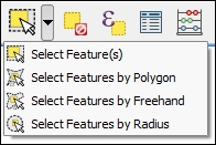
The first group of tools in the Attributes toolbar allows us to select features on the map using the mouse. The following screenshot shows the Select Feature(s) tool. We can select a single feature by clicking on it, or select multiple features by drawing a rectangle. The other tools can be used to select features by drawing different shapes (polygons, freehand areas, or circles) around the features. All features that intersect with the drawn shape are selected.
Selecting features with expressions
The second type of select tool is called Select by Expression, and it is also available in the Attribute toolbar. It selects features based on expressions that can contain references and functions that use feature attributes and/or geometry. The list of available functions in the center of the dialog is pretty long, but we can use the search box at the top of the list to filter it by name and find the function we are looking for faster. On the right-hand side of the window, we find the function help, which explains the functionality and how to use the function in an expression. The function list also shows the layer attribute fields, and by clicking on all unique or 10 samples, we can easily access their content. We can choose between creating a new selection or adding to or deleting from an existing selection. Additionally, we can choose to only select features from within an existing selection. Let's take a look at some example expressions that you can build on and use in your own work:
- Using the
lakes.shpfile in our sample data, we can, for example, select lakes with an area greater than 1,000 square miles by using a simple"AREA_MI" > 1000.0attribute query, as shown in the following screenshot. Alternatively, we can use geometry functions such as$area > (1000.0 * 27878400). Note that thelakes.shpCRS uses feet, and therefore we have to multiply by 27,878,400 to convert square feet to square miles.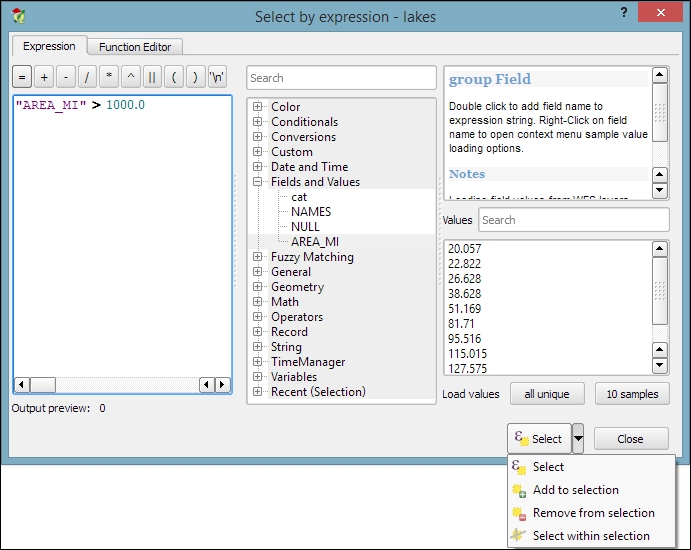
- We can also work with string functions, for example, to find lakes with long names (such as
length("NAMES") > 12) or lakes with names that containsorS(such aslower("NAMES") LIKE '%s%'); this function first converts the names to lowercase and then looks for any appearance ofs.
Selecting features using spatial queries
The third type of tool is called Spatial Query and allows us to select features in one layer based on their location relative to features in a second layer. These tools can be accessed by going to Vector | Research Tools | Select by location and Vector | Spatial Query | Spatial Query. Enable it in Plugin Manager if you cannot find it in the Vector menu. In general, we want to use the Spatial Query plugin as it supports a variety of spatial operations such as Crosses, Equals, Intersects, Is disjoint, Overlaps, Touches, and Contains, depending on the layer geometry type.
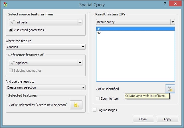
Let's test the Spatial Query plugin using railroads.shp and pipelines.shp from the sample data. For example, we might want to find all railroad features that cross a pipeline; therefore, we select the railroads layer, the Crosses operation, and the pipelines layer. After we've clicked on Apply, the plugin presents us with the query results. There is a list of IDs of the result features on the right-hand side of the window, as you can see in the next screenshot. Below this list, we can check the Zoom to item box, and QGIS will zoom into the feature that belongs to the selected ID. Additionally, the plugin offers buttons for direct saving of all the resulting features to a new layer:
Selecting features with the mouse
The first group of tools in the Attributes toolbar allows us to select features on the map using the mouse. The following screenshot shows the Select Feature(s) tool. We can select a single feature by clicking on it, or select multiple features by drawing a rectangle. The other tools can be used to select features by drawing different shapes (polygons, freehand areas, or circles) around the features. All features that intersect with the drawn shape are selected.

Selecting features with expressions
The second type of select tool is called Select by Expression, and it is also available in the Attribute toolbar. It selects features based on expressions that can contain references and functions that use feature attributes and/or geometry. The list of available functions in the center of the dialog is pretty long, but we can use the search box at the top of the list to filter it by name and find the function we are looking for faster. On the right-hand side of the window, we find the function help, which explains the functionality and how to use the function in an expression. The function list also shows the layer attribute fields, and by clicking on all unique or 10 samples, we can easily access their content. We can choose between creating a new selection or adding to or deleting from an existing selection. Additionally, we can choose to only select features from within an existing selection. Let's take a look at some example expressions that you can build on and use in your own work:
- Using the
lakes.shpfile in our sample data, we can, for example, select lakes with an area greater than 1,000 square miles by using a simple"AREA_MI" > 1000.0attribute query, as shown in the following screenshot. Alternatively, we can use geometry functions such as$area > (1000.0 * 27878400). Note that thelakes.shpCRS uses feet, and therefore we have to multiply by 27,878,400 to convert square feet to square miles.
- We can also work with string functions, for example, to find lakes with long names (such as
length("NAMES") > 12) or lakes with names that containsorS(such aslower("NAMES") LIKE '%s%'); this function first converts the names to lowercase and then looks for any appearance ofs.
Selecting features using spatial queries
The third type of tool is called Spatial Query and allows us to select features in one layer based on their location relative to features in a second layer. These tools can be accessed by going to Vector | Research Tools | Select by location and Vector | Spatial Query | Spatial Query. Enable it in Plugin Manager if you cannot find it in the Vector menu. In general, we want to use the Spatial Query plugin as it supports a variety of spatial operations such as Crosses, Equals, Intersects, Is disjoint, Overlaps, Touches, and Contains, depending on the layer geometry type.
Let's test the Spatial Query plugin using railroads.shp and pipelines.shp from the sample data. For example, we might want to find all railroad features that cross a pipeline; therefore, we select the railroads layer, the Crosses operation, and the pipelines layer. After we've clicked on Apply, the plugin presents us with the query results. There is a list of IDs of the result features on the right-hand side of the window, as you can see in the next screenshot. Below this list, we can check the Zoom to item box, and QGIS will zoom into the feature that belongs to the selected ID. Additionally, the plugin offers buttons for direct saving of all the resulting features to a new layer:

Selecting features with expressions
The second type of select tool is called Select by Expression, and it is also available in the Attribute toolbar. It selects features based on expressions that can contain references and functions that use feature attributes and/or geometry. The list of available functions in the center of the dialog is pretty long, but we can use the search box at the top of the list to filter it by name and find the function we are looking for faster. On the right-hand side of the window, we find the function help, which explains the functionality and how to use the function in an expression. The function list also shows the layer attribute fields, and by clicking on all unique or 10 samples, we can easily access their content. We can choose between creating a new selection or adding to or deleting from an existing selection. Additionally, we can choose to only select features from within an existing selection. Let's take a look at some example expressions that you can build on and use in your own work:
- Using the
lakes.shpfile in our sample data, we can, for example, select lakes with an area greater than 1,000 square miles by using a simple"AREA_MI" > 1000.0attribute query, as shown in the following screenshot. Alternatively, we can use geometry functions such as$area > (1000.0 * 27878400). Note that thelakes.shpCRS uses feet, and therefore we have to multiply by 27,878,400 to convert square feet to square miles.
- We can also work with string functions, for example, to find lakes with long names (such as
length("NAMES") > 12) or lakes with names that containsorS(such aslower("NAMES") LIKE '%s%'); this function first converts the names to lowercase and then looks for any appearance ofs.
Selecting features using spatial queries
The third type of tool is called Spatial Query and allows us to select features in one layer based on their location relative to features in a second layer. These tools can be accessed by going to Vector | Research Tools | Select by location and Vector | Spatial Query | Spatial Query. Enable it in Plugin Manager if you cannot find it in the Vector menu. In general, we want to use the Spatial Query plugin as it supports a variety of spatial operations such as Crosses, Equals, Intersects, Is disjoint, Overlaps, Touches, and Contains, depending on the layer geometry type.
Let's test the Spatial Query plugin using railroads.shp and pipelines.shp from the sample data. For example, we might want to find all railroad features that cross a pipeline; therefore, we select the railroads layer, the Crosses operation, and the pipelines layer. After we've clicked on Apply, the plugin presents us with the query results. There is a list of IDs of the result features on the right-hand side of the window, as you can see in the next screenshot. Below this list, we can check the Zoom to item box, and QGIS will zoom into the feature that belongs to the selected ID. Additionally, the plugin offers buttons for direct saving of all the resulting features to a new layer:

Editing vector geometries
Now that we know how to create and select features, we can take a closer look at the other tools in the Digitizing and Advanced Digitizing toolbars.
Using basic digitizing tools
This is the basic Digitizing toolbar:

The Digitizing toolbar contains tools that we can use to create and move features and nodes as well as delete, copy, cut, and paste features, as follows:
- The Add Feature tool allows us to create new features by placing feature nodes on the map, which are connected by straight lines.
- Similarly, the Add Circular String tool allows us to create features where consecutive nodes are connected by curved lines.
- With the Move Feature(s) tool, it is easy to move one or more features at once by dragging them to the new location.
- Similarly, the Node Tool feature allows us to move one or more nodes of the same feature. The first click activates the feature, while the second click selects the node. Hold the mouse key down to drag the node to its new location. Instead of moving only one node, we can also move an edge by clicking and dragging the line. Finally, we can select and move multiple nodes by holding down the Ctrl key.
- The Delete Selected, Cut Features, and Copy Features tools are active only if one or more layer features are selected. Similarly, Paste Features works only after a feature has been cut or copied.
Using advanced digitizing tools
The Advanced Digitizing toolbar offers very useful Undo and Redo functionalities as well as additional tools for more involved geometry editing, as shown in the following screenshot:

The Advanced Digitizing tools include the following:
- Rotate Feature(s) enables us to rotate one or more selected features around a central point.
- Using the Simplify Feature tool, we can simplify/generalize feature geometries by simply clicking on the feature and specifying a desired tolerance in the pop-up window, as shown in the following screenshot, where you can see the original geometry on the left-hand side and the simplified geometry on the right-hand side:

- The following tools can be used to modify polygons. They allow us to add rings, also known as holes, into existing polygons or add parts to them. The Fill Ring tool is similar to Add Ring, but instead of just creating a hole, it also creates a new feature that fills the hole. Of course, there are tools to delete rings and parts well.
- The Reshape Features tool can be used to alter the geometry of a feature by either cutting out or adding pieces. You can control the behavior by starting to draw the new form inside the original feature to add a piece, or by starting outside to cut out a piece, as shown in this example diagram:

- The Offset Curve tool is only available for lines and allows us to displace a line geometry by a given offset.
- The Split Features tool allows us to split one or more features into multiple features along a cut line. Similarly, Split Parts allows us to split a feature into multiple parts that still belong to the same multipolygon or multipolyline.
- The Merge Selected Features tool enables us to merge multiple features while keeping control over which feature's attributes will be available in the output feature.
- Similarly, Merge Attributes of Selected Features also lets us combine the attributes of multiple features but without merging them into one feature. Instead, all the original features remain as they were; the attribute values are updated.
- Finally, Rotate Point Symbols is available only for point layers with the Rotation field feature enabled (we will cover this feature in Chapter 5, Creating Great Maps).
Using snapping to enable topologically correct editing
One of the challenges of digitizing features by hand is avoiding undesired gaps or overlapping features. To make it easier to avoid these issues, QGIS offers a snapping functionality. To configure snapping, we go to Settings | Snapping options. The following screenshot shows how to enable snapping for the Current layer. Similarly, you can choose snapping modes for All layers or the Advanced mode, where you can control the settings for each layer separately. In the example shown in the following screenshot, we enable snapping To vertex. This means that digitizing tools will automatically snap to vertices/nodes of existing features in the current layer. Similarly, you can enable snapping To segment or To vertex and segment. When snapping is enabled during digitizing, you will notice bold cross-shaped markers appearing whenever you go close to a vertex or segment that can be snapped to:

Using basic digitizing tools
This is the basic Digitizing toolbar:

The Digitizing toolbar contains tools that we can use to create and move features and nodes as well as delete, copy, cut, and paste features, as follows:
- The Add Feature tool allows us to create new features by placing feature nodes on the map, which are connected by straight lines.
- Similarly, the Add Circular String tool allows us to create features where consecutive nodes are connected by curved lines.
- With the Move Feature(s) tool, it is easy to move one or more features at once by dragging them to the new location.
- Similarly, the Node Tool feature allows us to move one or more nodes of the same feature. The first click activates the feature, while the second click selects the node. Hold the mouse key down to drag the node to its new location. Instead of moving only one node, we can also move an edge by clicking and dragging the line. Finally, we can select and move multiple nodes by holding down the Ctrl key.
- The Delete Selected, Cut Features, and Copy Features tools are active only if one or more layer features are selected. Similarly, Paste Features works only after a feature has been cut or copied.
Using advanced digitizing tools
The Advanced Digitizing toolbar offers very useful Undo and Redo functionalities as well as additional tools for more involved geometry editing, as shown in the following screenshot:

The Advanced Digitizing tools include the following:
- Rotate Feature(s) enables us to rotate one or more selected features around a central point.
- Using the Simplify Feature tool, we can simplify/generalize feature geometries by simply clicking on the feature and specifying a desired tolerance in the pop-up window, as shown in the following screenshot, where you can see the original geometry on the left-hand side and the simplified geometry on the right-hand side:

- The following tools can be used to modify polygons. They allow us to add rings, also known as holes, into existing polygons or add parts to them. The Fill Ring tool is similar to Add Ring, but instead of just creating a hole, it also creates a new feature that fills the hole. Of course, there are tools to delete rings and parts well.
- The Reshape Features tool can be used to alter the geometry of a feature by either cutting out or adding pieces. You can control the behavior by starting to draw the new form inside the original feature to add a piece, or by starting outside to cut out a piece, as shown in this example diagram:

- The Offset Curve tool is only available for lines and allows us to displace a line geometry by a given offset.
- The Split Features tool allows us to split one or more features into multiple features along a cut line. Similarly, Split Parts allows us to split a feature into multiple parts that still belong to the same multipolygon or multipolyline.
- The Merge Selected Features tool enables us to merge multiple features while keeping control over which feature's attributes will be available in the output feature.
- Similarly, Merge Attributes of Selected Features also lets us combine the attributes of multiple features but without merging them into one feature. Instead, all the original features remain as they were; the attribute values are updated.
- Finally, Rotate Point Symbols is available only for point layers with the Rotation field feature enabled (we will cover this feature in Chapter 5, Creating Great Maps).
Using snapping to enable topologically correct editing
One of the challenges of digitizing features by hand is avoiding undesired gaps or overlapping features. To make it easier to avoid these issues, QGIS offers a snapping functionality. To configure snapping, we go to Settings | Snapping options. The following screenshot shows how to enable snapping for the Current layer. Similarly, you can choose snapping modes for All layers or the Advanced mode, where you can control the settings for each layer separately. In the example shown in the following screenshot, we enable snapping To vertex. This means that digitizing tools will automatically snap to vertices/nodes of existing features in the current layer. Similarly, you can enable snapping To segment or To vertex and segment. When snapping is enabled during digitizing, you will notice bold cross-shaped markers appearing whenever you go close to a vertex or segment that can be snapped to:

Using advanced digitizing tools
The Advanced Digitizing toolbar offers very useful Undo and Redo functionalities as well as additional tools for more involved geometry editing, as shown in the following screenshot:

The Advanced Digitizing tools include the following:
- Rotate Feature(s) enables us to rotate one or more selected features around a central point.
- Using the Simplify Feature tool, we can simplify/generalize feature geometries by simply clicking on the feature and specifying a desired tolerance in the pop-up window, as shown in the following screenshot, where you can see the original geometry on the left-hand side and the simplified geometry on the right-hand side:

- The following tools can be used to modify polygons. They allow us to add rings, also known as holes, into existing polygons or add parts to them. The Fill Ring tool is similar to Add Ring, but instead of just creating a hole, it also creates a new feature that fills the hole. Of course, there are tools to delete rings and parts well.
- The Reshape Features tool can be used to alter the geometry of a feature by either cutting out or adding pieces. You can control the behavior by starting to draw the new form inside the original feature to add a piece, or by starting outside to cut out a piece, as shown in this example diagram:

- The Offset Curve tool is only available for lines and allows us to displace a line geometry by a given offset.
- The Split Features tool allows us to split one or more features into multiple features along a cut line. Similarly, Split Parts allows us to split a feature into multiple parts that still belong to the same multipolygon or multipolyline.
- The Merge Selected Features tool enables us to merge multiple features while keeping control over which feature's attributes will be available in the output feature.
- Similarly, Merge Attributes of Selected Features also lets us combine the attributes of multiple features but without merging them into one feature. Instead, all the original features remain as they were; the attribute values are updated.
- Finally, Rotate Point Symbols is available only for point layers with the Rotation field feature enabled (we will cover this feature in Chapter 5, Creating Great Maps).
Using snapping to enable topologically correct editing
One of the challenges of digitizing features by hand is avoiding undesired gaps or overlapping features. To make it easier to avoid these issues, QGIS offers a snapping functionality. To configure snapping, we go to Settings | Snapping options. The following screenshot shows how to enable snapping for the Current layer. Similarly, you can choose snapping modes for All layers or the Advanced mode, where you can control the settings for each layer separately. In the example shown in the following screenshot, we enable snapping To vertex. This means that digitizing tools will automatically snap to vertices/nodes of existing features in the current layer. Similarly, you can enable snapping To segment or To vertex and segment. When snapping is enabled during digitizing, you will notice bold cross-shaped markers appearing whenever you go close to a vertex or segment that can be snapped to:

Using measuring tools
Another core functionality of any GIS is provided by measurement tools. In QGIS, we find the tools needed to measure lines, areas, and angles in the Attribute toolbar, as shown in this screenshot:
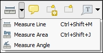
The measurements are updated continuously while we draw measurement lines, areas, or angles. When we draw a line with multiple segments, the tool shows the length of each segment as well as the total length of all the segments put together. To stop measuring, we can just right-click. If we want to change the measurement units from meters to feet or from degrees to radians, we can do this by going to Settings | Options | Map Tools.
Editing attributes
There are three main use cases of attribute editing:
- First, we might want to edit the attributes of a specific feature, for example, to fix a wrong name
- Second, we might want to edit the attributes of a group of features
- Third, we might want to change the attributes of all features within a layer
Editing attributes in the attribute table
All three use cases are covered by the functionality available through the attribute table. We can access it by going to Layer | Open Attribute Table, using the Open Attribute Table button present in the Attributes toolbar, or in the layer name context menu.
- To change an attribute value, we always have to enable editing first.
- Then, we can double-click on any cell in the attribute table to activate the input mode, as shown in the upper dialog of the following screenshot, where I am editing
NAME_2of the first feature:
- Pressing the Enter key confirms the change, but to save the new value permanently, we also have to click on the Save Edit(s) button or press Ctrl + S.
Besides the classic attribute table view, QGIS also supports a form view, which you can see in the lower dialog of the previous image. You can switch between these two views using the buttons in the bottom-right corner of the attribute table dialog.
Tip
In the attribute table, we also find tools for handling selections (from left to right, starting at the fourth button): Delete selected features, Select features using an expression, Unselect all, Move selection to top, Invert selection, Pan map to the selected rows, Zoom map to the selected rows, and Copy selected rows to clipboard. Another way to select features in the attribute table is by clicking on the row number.
The next two buttons allow us to add and remove columns. When we click on the Delete column button, we get a list of columns to choose from. Similarly, the New column button brings up a dialog that we can use to specify the name and data type of the new column.
Editing attributes in the feature form
Another option to edit the attributes of one feature is to open the attribute form directly by clicking on the feature on the map using the Identify tool. By default, the Identify tool displays the attribute values in read mode, but we can enable the Auto open form option in the Identify Results panel, as shown here:
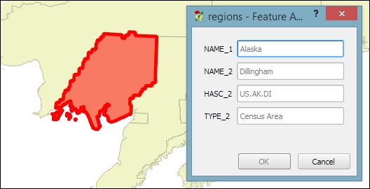
What you can see in the previous screenshot is the default feature attributes form that QGIS creates automatically, but we are not limited to this basic form. By going to Layer Properties | Fields section, we can configure the look and feel of the form in greater detail. The Attribute editor layout options are (in an increasing level of complexity) autogenerate, Drag and drop designer, and providing a .ui file. These options are described in detail as follows.
Creating a feature form using autogenerate
Autogenerate is the most basic option. You can assign a specific Edit widget and Alias for each field; this will replace the default input field and label in the form. For this example, we use the following edit widget types:
- Text Edit supports inserting one or more lines of text.
- Unique Values creates a drop-down list that allows the user to select one of the values that have already been used in the attribute table. If the Editable option is activated, the drop-down list is replaced by a text edit widget with autocompletion support.
- Range creates an edit widget for numerical values from a specific range.
Note
For the complete list of available Edit widget types, refer to the user manual at http://docs.qgis.org/2.2/en/docs/user_manual/working_with_vector/vector_properties.html#fields-menu.
Designing a feature form using drag and drop designer
This allows more control over the form layout. As you can see in the next screenshot, the designer enables us to create tabs within the form and also makes it possible to change the order of the form fields. The workflow is as follows:
- Click on the plus button to add one or more tabs (for example, a Region tab, as shown in the following screenshot).
- On the left-hand side of the dialog, select the field that you want to add to the form.
- On the right-hand side, select the tab to which you want to add the field.
- Click on the button with the icon of an arrow pointing to the right to add the selected field to the selected tab.
- You can reorder the fields in the form using the up and down arrow buttons or, as the name suggests, by dragging and dropping the fields up or down:

Designing a feature form using a .ui file
This is the most advanced option. It enables you to use a Qt user interface designed using, for example, the Qt Designer software. This allows a great deal of freedom in designing the form layout and behavior.
Note
Creating .ui files is out of the scope of this book, but you can find more information about it at http://docs.qgis.org/2.2/en/docs/training_manual/create_vector_data/forms.html#hard-fa-creating-a-new-form.
Calculating new attribute values
If we want to change the attributes of multiple or all features in a layer, editing them manually usually isn't an option. This is what the Field calculator is good for. We can access it using the Open field calculator button in the attribute table, or by pressing Ctrl + I. In the Field calculator, we can choose to update only the selected features or update all the features in the layer. Besides updating an existing field, we can also create a new field. The function list is the same one that we explored when we selected features by expression. We can use any of the functions and variables in this list to populate a new field or update an existing one. Here are some example expressions that are often used:
- We can create a sequential
idcolumn using the@row_numbervariable, which populates a column with row numbers, as shown in the following screenshot:
- Another common use case is calculating a line's length or a polygon's area using the
$lengthand$areageometry functions, respectively - Similarly, we can get point coordinates using
$xand$y - If we want to get the start point or end point of a line, we can use
$x_at(0)and$y_at(0), or$x_at(-1)and$y_at(-1), respectively
An alternative to the Field calculator—especially if you already know the formula you want to use—is the field calculator bar, which you can find directly in the Attribute table dialog right below the toolbar. In the next screenshot, you can see an example that calculates the area of all census areas (use the New Field button to add a Decimal number field called CENSUSAREA first). This example uses a CASE WHEN – THEN – END expression to check whether the value of TYPE_2 is Census Area:
CASE WHEN TYPE_2 = 'Census Area' THEN $area / 27878400 END
Tip
An alternative solution would be to use the if() function instead. If you use the CENSUSAREA attribute as the third parameter (which defines the value that is returned if the condition evaluates to false), the expression will only update those rows in which TYPE_2 is Census Area and leave the other rows unchanged:
if(TYPE_2 = 'Census Area', $area / 27878400, CENSUSAREA)
Alternatively, you can use NULL as a third parameter which will overwrite all rows where TYPE_2 does not equal Census Area with NULL:
if(TYPE_2 = 'Census Area', $area / 27878400, NULL)
Enter the formula and click on the Update All button to execute it:
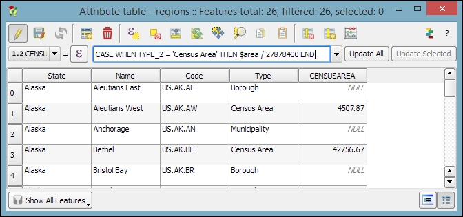
Since it is not possible to directly change a field data type in a Shapefile or SpatiaLite attribute table, the field calculator and calculator bar are also used to create new fields with the desired properties and then populate them with the values from the original column.
Editing attributes in the attribute table
All three use cases are covered by the functionality available through the attribute table. We can access it by going to Layer | Open Attribute Table, using the Open Attribute Table button present in the Attributes toolbar, or in the layer name context menu.
- To change an attribute value, we always have to enable editing first.
- Then, we can double-click on any cell in the attribute table to activate the input mode, as shown in the upper dialog of the following screenshot, where I am editing
NAME_2of the first feature:
- Pressing the Enter key confirms the change, but to save the new value permanently, we also have to click on the Save Edit(s) button or press Ctrl + S.
Besides the classic attribute table view, QGIS also supports a form view, which you can see in the lower dialog of the previous image. You can switch between these two views using the buttons in the bottom-right corner of the attribute table dialog.
Tip
In the attribute table, we also find tools for handling selections (from left to right, starting at the fourth button): Delete selected features, Select features using an expression, Unselect all, Move selection to top, Invert selection, Pan map to the selected rows, Zoom map to the selected rows, and Copy selected rows to clipboard. Another way to select features in the attribute table is by clicking on the row number.
The next two buttons allow us to add and remove columns. When we click on the Delete column button, we get a list of columns to choose from. Similarly, the New column button brings up a dialog that we can use to specify the name and data type of the new column.
Editing attributes in the feature form
Another option to edit the attributes of one feature is to open the attribute form directly by clicking on the feature on the map using the Identify tool. By default, the Identify tool displays the attribute values in read mode, but we can enable the Auto open form option in the Identify Results panel, as shown here:

What you can see in the previous screenshot is the default feature attributes form that QGIS creates automatically, but we are not limited to this basic form. By going to Layer Properties | Fields section, we can configure the look and feel of the form in greater detail. The Attribute editor layout options are (in an increasing level of complexity) autogenerate, Drag and drop designer, and providing a .ui file. These options are described in detail as follows.
Creating a feature form using autogenerate
Autogenerate is the most basic option. You can assign a specific Edit widget and Alias for each field; this will replace the default input field and label in the form. For this example, we use the following edit widget types:
- Text Edit supports inserting one or more lines of text.
- Unique Values creates a drop-down list that allows the user to select one of the values that have already been used in the attribute table. If the Editable option is activated, the drop-down list is replaced by a text edit widget with autocompletion support.
- Range creates an edit widget for numerical values from a specific range.
Note
For the complete list of available Edit widget types, refer to the user manual at http://docs.qgis.org/2.2/en/docs/user_manual/working_with_vector/vector_properties.html#fields-menu.
Designing a feature form using drag and drop designer
This allows more control over the form layout. As you can see in the next screenshot, the designer enables us to create tabs within the form and also makes it possible to change the order of the form fields. The workflow is as follows:
- Click on the plus button to add one or more tabs (for example, a Region tab, as shown in the following screenshot).
- On the left-hand side of the dialog, select the field that you want to add to the form.
- On the right-hand side, select the tab to which you want to add the field.
- Click on the button with the icon of an arrow pointing to the right to add the selected field to the selected tab.
- You can reorder the fields in the form using the up and down arrow buttons or, as the name suggests, by dragging and dropping the fields up or down:

Designing a feature form using a .ui file
This is the most advanced option. It enables you to use a Qt user interface designed using, for example, the Qt Designer software. This allows a great deal of freedom in designing the form layout and behavior.
Note
Creating .ui files is out of the scope of this book, but you can find more information about it at http://docs.qgis.org/2.2/en/docs/training_manual/create_vector_data/forms.html#hard-fa-creating-a-new-form.
Calculating new attribute values
If we want to change the attributes of multiple or all features in a layer, editing them manually usually isn't an option. This is what the Field calculator is good for. We can access it using the Open field calculator button in the attribute table, or by pressing Ctrl + I. In the Field calculator, we can choose to update only the selected features or update all the features in the layer. Besides updating an existing field, we can also create a new field. The function list is the same one that we explored when we selected features by expression. We can use any of the functions and variables in this list to populate a new field or update an existing one. Here are some example expressions that are often used:
- We can create a sequential
idcolumn using the@row_numbervariable, which populates a column with row numbers, as shown in the following screenshot:
- Another common use case is calculating a line's length or a polygon's area using the
$lengthand$areageometry functions, respectively - Similarly, we can get point coordinates using
$xand$y - If we want to get the start point or end point of a line, we can use
$x_at(0)and$y_at(0), or$x_at(-1)and$y_at(-1), respectively
An alternative to the Field calculator—especially if you already know the formula you want to use—is the field calculator bar, which you can find directly in the Attribute table dialog right below the toolbar. In the next screenshot, you can see an example that calculates the area of all census areas (use the New Field button to add a Decimal number field called CENSUSAREA first). This example uses a CASE WHEN – THEN – END expression to check whether the value of TYPE_2 is Census Area:
CASE WHEN TYPE_2 = 'Census Area' THEN $area / 27878400 END
Tip
An alternative solution would be to use the if() function instead. If you use the CENSUSAREA attribute as the third parameter (which defines the value that is returned if the condition evaluates to false), the expression will only update those rows in which TYPE_2 is Census Area and leave the other rows unchanged:
if(TYPE_2 = 'Census Area', $area / 27878400, CENSUSAREA)
Alternatively, you can use NULL as a third parameter which will overwrite all rows where TYPE_2 does not equal Census Area with NULL:
if(TYPE_2 = 'Census Area', $area / 27878400, NULL)
Enter the formula and click on the Update All button to execute it:

Since it is not possible to directly change a field data type in a Shapefile or SpatiaLite attribute table, the field calculator and calculator bar are also used to create new fields with the desired properties and then populate them with the values from the original column.
Editing attributes in the feature form
Another option to edit the attributes of one feature is to open the attribute form directly by clicking on the feature on the map using the Identify tool. By default, the Identify tool displays the attribute values in read mode, but we can enable the Auto open form option in the Identify Results panel, as shown here:

What you can see in the previous screenshot is the default feature attributes form that QGIS creates automatically, but we are not limited to this basic form. By going to Layer Properties | Fields section, we can configure the look and feel of the form in greater detail. The Attribute editor layout options are (in an increasing level of complexity) autogenerate, Drag and drop designer, and providing a .ui file. These options are described in detail as follows.
Creating a feature form using autogenerate
Autogenerate is the most basic option. You can assign a specific Edit widget and Alias for each field; this will replace the default input field and label in the form. For this example, we use the following edit widget types:
- Text Edit supports inserting one or more lines of text.
- Unique Values creates a drop-down list that allows the user to select one of the values that have already been used in the attribute table. If the Editable option is activated, the drop-down list is replaced by a text edit widget with autocompletion support.
- Range creates an edit widget for numerical values from a specific range.
Note
For the complete list of available Edit widget types, refer to the user manual at http://docs.qgis.org/2.2/en/docs/user_manual/working_with_vector/vector_properties.html#fields-menu.
Designing a feature form using drag and drop designer
This allows more control over the form layout. As you can see in the next screenshot, the designer enables us to create tabs within the form and also makes it possible to change the order of the form fields. The workflow is as follows:
- Click on the plus button to add one or more tabs (for example, a Region tab, as shown in the following screenshot).
- On the left-hand side of the dialog, select the field that you want to add to the form.
- On the right-hand side, select the tab to which you want to add the field.
- Click on the button with the icon of an arrow pointing to the right to add the selected field to the selected tab.
- You can reorder the fields in the form using the up and down arrow buttons or, as the name suggests, by dragging and dropping the fields up or down:

Designing a feature form using a .ui file
This is the most advanced option. It enables you to use a Qt user interface designed using, for example, the Qt Designer software. This allows a great deal of freedom in designing the form layout and behavior.
Note
Creating .ui files is out of the scope of this book, but you can find more information about it at http://docs.qgis.org/2.2/en/docs/training_manual/create_vector_data/forms.html#hard-fa-creating-a-new-form.
Calculating new attribute values
If we want to change the attributes of multiple or all features in a layer, editing them manually usually isn't an option. This is what the Field calculator is good for. We can access it using the Open field calculator button in the attribute table, or by pressing Ctrl + I. In the Field calculator, we can choose to update only the selected features or update all the features in the layer. Besides updating an existing field, we can also create a new field. The function list is the same one that we explored when we selected features by expression. We can use any of the functions and variables in this list to populate a new field or update an existing one. Here are some example expressions that are often used:
- We can create a sequential
idcolumn using the@row_numbervariable, which populates a column with row numbers, as shown in the following screenshot:
- Another common use case is calculating a line's length or a polygon's area using the
$lengthand$areageometry functions, respectively - Similarly, we can get point coordinates using
$xand$y - If we want to get the start point or end point of a line, we can use
$x_at(0)and$y_at(0), or$x_at(-1)and$y_at(-1), respectively
An alternative to the Field calculator—especially if you already know the formula you want to use—is the field calculator bar, which you can find directly in the Attribute table dialog right below the toolbar. In the next screenshot, you can see an example that calculates the area of all census areas (use the New Field button to add a Decimal number field called CENSUSAREA first). This example uses a CASE WHEN – THEN – END expression to check whether the value of TYPE_2 is Census Area:
CASE WHEN TYPE_2 = 'Census Area' THEN $area / 27878400 END
Tip
An alternative solution would be to use the if() function instead. If you use the CENSUSAREA attribute as the third parameter (which defines the value that is returned if the condition evaluates to false), the expression will only update those rows in which TYPE_2 is Census Area and leave the other rows unchanged:
if(TYPE_2 = 'Census Area', $area / 27878400, CENSUSAREA)
Alternatively, you can use NULL as a third parameter which will overwrite all rows where TYPE_2 does not equal Census Area with NULL:
if(TYPE_2 = 'Census Area', $area / 27878400, NULL)
Enter the formula and click on the Update All button to execute it:

Since it is not possible to directly change a field data type in a Shapefile or SpatiaLite attribute table, the field calculator and calculator bar are also used to create new fields with the desired properties and then populate them with the values from the original column.
Creating a feature form using autogenerate
Autogenerate is the most basic option. You can assign a specific Edit widget and Alias for each field; this will replace the default input field and label in the form. For this example, we use the following edit widget types:
- Text Edit supports inserting one or more lines of text.
- Unique Values creates a drop-down list that allows the user to select one of the values that have already been used in the attribute table. If the Editable option is activated, the drop-down list is replaced by a text edit widget with autocompletion support.
- Range creates an edit widget for numerical values from a specific range.
Note
For the complete list of available Edit widget types, refer to the user manual at http://docs.qgis.org/2.2/en/docs/user_manual/working_with_vector/vector_properties.html#fields-menu.
Designing a feature form using drag and drop designer
This allows more control over the form layout. As you can see in the next screenshot, the designer enables us to create tabs within the form and also makes it possible to change the order of the form fields. The workflow is as follows:
- Click on the plus button to add one or more tabs (for example, a Region tab, as shown in the following screenshot).
- On the left-hand side of the dialog, select the field that you want to add to the form.
- On the right-hand side, select the tab to which you want to add the field.
- Click on the button with the icon of an arrow pointing to the right to add the selected field to the selected tab.
- You can reorder the fields in the form using the up and down arrow buttons or, as the name suggests, by dragging and dropping the fields up or down:

Designing a feature form using a .ui file
This is the most advanced option. It enables you to use a Qt user interface designed using, for example, the Qt Designer software. This allows a great deal of freedom in designing the form layout and behavior.
Note
Creating .ui files is out of the scope of this book, but you can find more information about it at http://docs.qgis.org/2.2/en/docs/training_manual/create_vector_data/forms.html#hard-fa-creating-a-new-form.
If we want to change the attributes of multiple or all features in a layer, editing them manually usually isn't an option. This is what the Field calculator is good for. We can access it using the Open field calculator button in the attribute table, or by pressing Ctrl + I. In the Field calculator, we can choose to update only the selected features or update all the features in the layer. Besides updating an existing field, we can also create a new field. The function list is the same one that we explored when we selected features by expression. We can use any of the functions and variables in this list to populate a new field or update an existing one. Here are some example expressions that are often used:
- We can create a sequential
idcolumn using the@row_numbervariable, which populates a column with row numbers, as shown in the following screenshot:
- Another common use case is calculating a line's length or a polygon's area using the
$lengthand$areageometry functions, respectively - Similarly, we can get point coordinates using
$xand$y - If we want to get the start point or end point of a line, we can use
$x_at(0)and$y_at(0), or$x_at(-1)and$y_at(-1), respectively
An alternative to the Field calculator—especially if you already know the formula you want to use—is the field calculator bar, which you can find directly in the Attribute table dialog right below the toolbar. In the next screenshot, you can see an example that calculates the area of all census areas (use the New Field button to add a Decimal number field called CENSUSAREA first). This example uses a CASE WHEN – THEN – END expression to check whether the value of TYPE_2 is Census Area:
CASE WHEN TYPE_2 = 'Census Area' THEN $area / 27878400 END
Tip
An alternative solution would be to use the if() function instead. If you use the CENSUSAREA attribute as the third parameter (which defines the value that is returned if the condition evaluates to false), the expression will only update those rows in which TYPE_2 is Census Area and leave the other rows unchanged:
if(TYPE_2 = 'Census Area', $area / 27878400, CENSUSAREA)
Alternatively, you can use NULL as a third parameter which will overwrite all rows where TYPE_2 does not equal Census Area with NULL:
if(TYPE_2 = 'Census Area', $area / 27878400, NULL)
Enter the formula and click on the Update All button to execute it:

Since it is not possible to directly change a field data type in a Shapefile or SpatiaLite attribute table, the field calculator and calculator bar are also used to create new fields with the desired properties and then populate them with the values from the original column.
Designing a feature form using drag and drop designer
This allows more control over the form layout. As you can see in the next screenshot, the designer enables us to create tabs within the form and also makes it possible to change the order of the form fields. The workflow is as follows:
- Click on the plus button to add one or more tabs (for example, a Region tab, as shown in the following screenshot).
- On the left-hand side of the dialog, select the field that you want to add to the form.
- On the right-hand side, select the tab to which you want to add the field.
- Click on the button with the icon of an arrow pointing to the right to add the selected field to the selected tab.
- You can reorder the fields in the form using the up and down arrow buttons or, as the name suggests, by dragging and dropping the fields up or down:

Designing a feature form using a .ui file
This is the most advanced option. It enables you to use a Qt user interface designed using, for example, the Qt Designer software. This allows a great deal of freedom in designing the form layout and behavior.
Note
Creating .ui files is out of the scope of this book, but you can find more information about it at http://docs.qgis.org/2.2/en/docs/training_manual/create_vector_data/forms.html#hard-fa-creating-a-new-form.
If we want to change the attributes of multiple or all features in a layer, editing them manually usually isn't an option. This is what the Field calculator is good for. We can access it using the Open field calculator button in the attribute table, or by pressing Ctrl + I. In the Field calculator, we can choose to update only the selected features or update all the features in the layer. Besides updating an existing field, we can also create a new field. The function list is the same one that we explored when we selected features by expression. We can use any of the functions and variables in this list to populate a new field or update an existing one. Here are some example expressions that are often used:
- We can create a sequential
idcolumn using the@row_numbervariable, which populates a column with row numbers, as shown in the following screenshot:
- Another common use case is calculating a line's length or a polygon's area using the
$lengthand$areageometry functions, respectively - Similarly, we can get point coordinates using
$xand$y - If we want to get the start point or end point of a line, we can use
$x_at(0)and$y_at(0), or$x_at(-1)and$y_at(-1), respectively
An alternative to the Field calculator—especially if you already know the formula you want to use—is the field calculator bar, which you can find directly in the Attribute table dialog right below the toolbar. In the next screenshot, you can see an example that calculates the area of all census areas (use the New Field button to add a Decimal number field called CENSUSAREA first). This example uses a CASE WHEN – THEN – END expression to check whether the value of TYPE_2 is Census Area:
CASE WHEN TYPE_2 = 'Census Area' THEN $area / 27878400 END
Tip
An alternative solution would be to use the if() function instead. If you use the CENSUSAREA attribute as the third parameter (which defines the value that is returned if the condition evaluates to false), the expression will only update those rows in which TYPE_2 is Census Area and leave the other rows unchanged:
if(TYPE_2 = 'Census Area', $area / 27878400, CENSUSAREA)
Alternatively, you can use NULL as a third parameter which will overwrite all rows where TYPE_2 does not equal Census Area with NULL:
if(TYPE_2 = 'Census Area', $area / 27878400, NULL)
Enter the formula and click on the Update All button to execute it:

Since it is not possible to directly change a field data type in a Shapefile or SpatiaLite attribute table, the field calculator and calculator bar are also used to create new fields with the desired properties and then populate them with the values from the original column.
Designing a feature form using a .ui file
This is the most advanced option. It enables you to use a Qt user interface designed using, for example, the Qt Designer software. This allows a great deal of freedom in designing the form layout and behavior.
Note
Creating .ui files is out of the scope of this book, but you can find more information about it at http://docs.qgis.org/2.2/en/docs/training_manual/create_vector_data/forms.html#hard-fa-creating-a-new-form.
If we want to change the attributes of multiple or all features in a layer, editing them manually usually isn't an option. This is what the Field calculator is good for. We can access it using the Open field calculator button in the attribute table, or by pressing Ctrl + I. In the Field calculator, we can choose to update only the selected features or update all the features in the layer. Besides updating an existing field, we can also create a new field. The function list is the same one that we explored when we selected features by expression. We can use any of the functions and variables in this list to populate a new field or update an existing one. Here are some example expressions that are often used:
- We can create a sequential
idcolumn using the@row_numbervariable, which populates a column with row numbers, as shown in the following screenshot:
- Another common use case is calculating a line's length or a polygon's area using the
$lengthand$areageometry functions, respectively - Similarly, we can get point coordinates using
$xand$y - If we want to get the start point or end point of a line, we can use
$x_at(0)and$y_at(0), or$x_at(-1)and$y_at(-1), respectively
An alternative to the Field calculator—especially if you already know the formula you want to use—is the field calculator bar, which you can find directly in the Attribute table dialog right below the toolbar. In the next screenshot, you can see an example that calculates the area of all census areas (use the New Field button to add a Decimal number field called CENSUSAREA first). This example uses a CASE WHEN – THEN – END expression to check whether the value of TYPE_2 is Census Area:
CASE WHEN TYPE_2 = 'Census Area' THEN $area / 27878400 END
Tip
An alternative solution would be to use the if() function instead. If you use the CENSUSAREA attribute as the third parameter (which defines the value that is returned if the condition evaluates to false), the expression will only update those rows in which TYPE_2 is Census Area and leave the other rows unchanged:
if(TYPE_2 = 'Census Area', $area / 27878400, CENSUSAREA)
Alternatively, you can use NULL as a third parameter which will overwrite all rows where TYPE_2 does not equal Census Area with NULL:
if(TYPE_2 = 'Census Area', $area / 27878400, NULL)
Enter the formula and click on the Update All button to execute it:

Since it is not possible to directly change a field data type in a Shapefile or SpatiaLite attribute table, the field calculator and calculator bar are also used to create new fields with the desired properties and then populate them with the values from the original column.
Calculating new attribute values
If we want to change the attributes of multiple or all features in a layer, editing them manually usually isn't an option. This is what the Field calculator is good for. We can access it using the Open field calculator button in the attribute table, or by pressing Ctrl + I. In the Field calculator, we can choose to update only the selected features or update all the features in the layer. Besides updating an existing field, we can also create a new field. The function list is the same one that we explored when we selected features by expression. We can use any of the functions and variables in this list to populate a new field or update an existing one. Here are some example expressions that are often used:
- We can create a sequential
idcolumn using the@row_numbervariable, which populates a column with row numbers, as shown in the following screenshot:
- Another common use case is calculating a line's length or a polygon's area using the
$lengthand$areageometry functions, respectively - Similarly, we can get point coordinates using
$xand$y - If we want to get the start point or end point of a line, we can use
$x_at(0)and$y_at(0), or$x_at(-1)and$y_at(-1), respectively
An alternative to the Field calculator—especially if you already know the formula you want to use—is the field calculator bar, which you can find directly in the Attribute table dialog right below the toolbar. In the next screenshot, you can see an example that calculates the area of all census areas (use the New Field button to add a Decimal number field called CENSUSAREA first). This example uses a CASE WHEN – THEN – END expression to check whether the value of TYPE_2 is Census Area:
CASE WHEN TYPE_2 = 'Census Area' THEN $area / 27878400 END
Tip
An alternative solution would be to use the if() function instead. If you use the CENSUSAREA attribute as the third parameter (which defines the value that is returned if the condition evaluates to false), the expression will only update those rows in which TYPE_2 is Census Area and leave the other rows unchanged:
if(TYPE_2 = 'Census Area', $area / 27878400, CENSUSAREA)
Alternatively, you can use NULL as a third parameter which will overwrite all rows where TYPE_2 does not equal Census Area with NULL:
if(TYPE_2 = 'Census Area', $area / 27878400, NULL)
Enter the formula and click on the Update All button to execute it:

Since it is not possible to directly change a field data type in a Shapefile or SpatiaLite attribute table, the field calculator and calculator bar are also used to create new fields with the desired properties and then populate them with the values from the original column.
Reprojecting and converting vector and raster data
In Chapter 2, Viewing Spatial Data, we talked about CRS and the fact that QGIS offers on the fly reprojection to display spatial datasets, which are stored in different CRS, in the same map. Still, in some cases, we might want to permanently reproject a dataset, for example, to geoprocess it later on.
In QGIS, reprojecting a vector or raster layer is done by simply saving it with a new CRS. We can save a layer by going to Layer | Save as... or using Save as… in the layer name context menu. Pick a target file format and filename, and then click on the Select CRS button beside the CRS drop-down field to pick a new CRS.
Besides changing the CRS, the main use case of the Save vector/raster layer dialog, as depicted in the following screenshot, is conversion between different file formats. For example, we can load a Shapefile and export it as GeoJSON, MapInfo MIF, CSV, and so on, or the other way around.
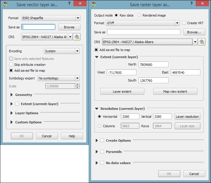
The Save raster layer dialog is also a convenient way to clip/crop rasters by a bounding box, since we can specify which Extent we want to save.
Furthermore, the Save vector layer dialog features a Save only selected features option, which enables us to save only selected features instead of all features of the layer (this option is active only if there are actually some selected features in the layer).
Tip
Enabling Add saved file to map is very convenient because it saves us the effort of going and loading the new file manually after it has been saved.
Joining tabular data
In many real-life situations, we get additional non-spatial data in the form of spreadsheets or text files. The good news is that we can load XLS files by simply dragging them into QGIS from the file browser or using Add Vector Layer. Don't let the wording fool you! It really works without any geometry data in the file. The file can even contain more than one table. You will see the following dialog, which lets you choose which table (or tables) you want to load:

QGIS will automatically recognize the names and data types of columns in an XLS table. It's quite easy to tell because numerical values are aligned to the right in the attribute table, as shown in this screenshot:
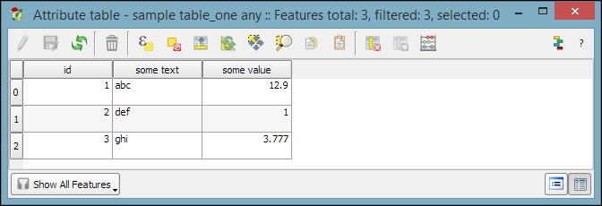
We can also load tabular data from delimited text files, as we saw in Chapter 2, Viewing Spatial Data, when we loaded a point layer from a delimited text file. To load a delimited text file that contains only tabular data but no geometry information, we just need to enable the No geometry (attribute table only) option.
Setting up a join in Layer Properties
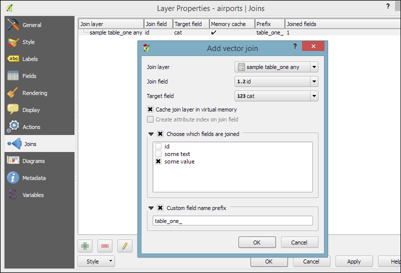
After loading the tabular data from either the spreadsheet or text file, we can continue to join this non-spatial data to a vector layer (for instance, our airports.shp dataset, as shown in the following example). To do this, we go to the vector's Layer Properties | Joins section. Here, we can add a new join by clicking on the green plus button. All we have to do is select the tabular Join layer and Join field (of the tabular layer), which will contain values that match those in the Target field (of the vector layer). Additionally, we can—if we want to—select a subset of the fields to be joined by enabling the Choose which fields are joined option. For example, the settings shown in the following screenshot will add only the some value field. Additionally, we use a Custom field name prefix instead of using the entire join layer name, which would be the default option.
Checking join results in the attribute table
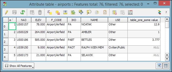
Once the join is added, we can see the extended attribute table and use the new appended attributes (as shown in the following screenshot) for styling and labeling. The way joins work in QGIS is as follows: the join layer's attributes are appended to the original layer's attribute table. The number of features in the original layer is not changed. Whenever there is a match between the join and the target field, the attribute value is filled in; otherwise, you see NULL entries.
You can save the joined layer permanently using Save as… to create the new file.
Setting up a join in Layer Properties
After loading the tabular data from either the spreadsheet or text file, we can continue to join this non-spatial data to a vector layer (for instance, our airports.shp dataset, as shown in the following example). To do this, we go to the vector's Layer Properties | Joins section. Here, we can add a new join by clicking on the green plus button. All we have to do is select the tabular Join layer and Join field (of the tabular layer), which will contain values that match those in the Target field (of the vector layer). Additionally, we can—if we want to—select a subset of the fields to be joined by enabling the Choose which fields are joined option. For example, the settings shown in the following screenshot will add only the some value field. Additionally, we use a Custom field name prefix instead of using the entire join layer name, which would be the default option.

Checking join results in the attribute table
Once the join is added, we can see the extended attribute table and use the new appended attributes (as shown in the following screenshot) for styling and labeling. The way joins work in QGIS is as follows: the join layer's attributes are appended to the original layer's attribute table. The number of features in the original layer is not changed. Whenever there is a match between the join and the target field, the attribute value is filled in; otherwise, you see NULL entries.

You can save the joined layer permanently using Save as… to create the new file.
Checking join results in the attribute table
Once the join is added, we can see the extended attribute table and use the new appended attributes (as shown in the following screenshot) for styling and labeling. The way joins work in QGIS is as follows: the join layer's attributes are appended to the original layer's attribute table. The number of features in the original layer is not changed. Whenever there is a match between the join and the target field, the attribute value is filled in; otherwise, you see NULL entries.

You can save the joined layer permanently using Save as… to create the new file.
Using temporary scratch layers
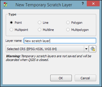
When you just want to quickly draw some features on the map, temporary scratch layers are a great way of doing that without having to worry about file formats and locations for your temporary data. Go to Layer | Create Layer | New Temporary Scratch Layer... to create a new temporary scratch layer. As you can see in the following screenshot, all we need to do to configure this temporary layer is pick a Type for the geometry, a Layer name, and a CRS. Once the layer is created, we can add features and attributes as we would with any other vector layer:
As the name suggests, temporary scratch layers are temporary. This means that they will vanish when you close the project.
Tip
If you want to preserve the data of your temporary layers, you can either use Save as... to create a file or install the Memory Layer Saver plugin, which will make layers with memory data providers (such as temporary scratch layers) persistent so that they are restored when a project is closed and reopened. The memory provider data is saved in a portable binary format that is saved with the .mldata extension alongside the project file.
Checking for topological errors and fixing them
Sometimes, the data that we receive from different sources or data that results from a chain of spatial processing steps can have problems. Topological errors can be particularly annoying, since they can lead to a multitude of different problems when using the data for analysis and further spatial processing. Therefore, it is important to have tools that can check data for topological errors and to know ways to fix discovered errors.
Finding errors with the Topology Checker
In QGIS, we can use the Topology Checker plugin; it is installed by default and is accessible via the Vector menu Topology Checker entry (if you cannot find the menu entry, you might have to enable the plugin in Plugin Manager). When the plugin is activated, it adds a Topology Checker Panel to the QGIS window. This panel can be used to configure and run different topology checks and will list the detected errors.
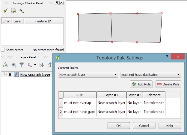
To see the Topology Checker in action, we create a temporary scratch layer with polygon geometries and digitize some polygons, as shown in the following screenshot. Make sure you use snapping to create polygons that touch but don't overlap. These could, for example, represent a group of row houses. When the polygons are ready, we can set up the topology rules we want to check for. Click on the Configure button in Topology Checker Panel to open the Topology Rule Settings dialog. Here, we can manage all the topology rules for our project data. For example, in the following screenshot, you can see the rules we might want to configure for our polygon layer, including these:
- Polygons must not overlap each other
- There must not be gaps between polygons
- There shouldn't be any duplicate geometries
Once the rules are set up, we can close the settings dialog and click on the Validate All button in Topology Checker Panel to start running the topology rule checks. If you have been careful while creating the polygons, the checker will not find any errors and the status at the bottom of Topology Checker Panel will display this message: 0 errors were found. Let's change that by introducing some topology errors.
For example, if we move one vertex so that two polygons end up overlapping each other and then click on Validate All, we get the error shown in the next screenshot. Note that the error type and the affected layer and feature are displayed in Topology Checker Panel. Additionally, since the Show errors option is enabled, the problematic geometry part is highlighted in red on the map:

Of course, it is also possible to create rules that describe the relationship between features in different layers. For example, the following screenshot shows a point and a polygon layer where the rules state that each point should be inside a polygon and each polygon should contain a point:
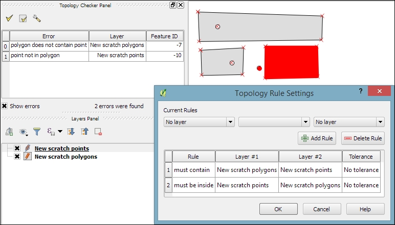
Selecting an error from the list of errors in the panel centres the map on the problematic location so that we can start fixing it, for example, by moving the lone point into the empty polygon.
Fixing invalid geometry errors
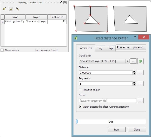
Sometimes, fixing all errors manually can be a lot of work. Luckily, certain errors can be addressed automatically. For example, the common error of self-intersecting polygons, which cause invalid geometry errors (as illustrated in the following screenshot), is often the result of intersecting polygon nodes or edges. These issues can often be resolved using a buffer tool (for example, Fixed distance buffer in the Processing Toolbox, which we will discuss in more detail in Chapter 4, Spatial Analysis) with the buffer Distance set to 0. Buffering will, for example, fix the self-intersecting polygon on the left-hand side of the following screenshot by removing the self-intersecting nodes and constructing a valid polygon with a hole (as depicted on the right-hand side):
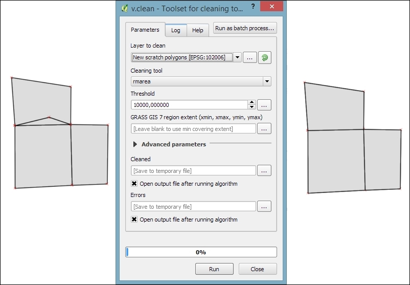
Another common issue that can be fixed automatically is so-called sliver polygons. These are small, and often quite thin, polygons that can be the result of spatial processes such as intersection operations. To get rid of these sliver polygons, we can use the v.clean tool with the Cleaning tool option set to rmarea (meaning "remove area"), which is also available through the Processing Toolbox. In the example shown in this screenshot, the Threshold value of 10000 tells the tool to remove all polygons with an area less than 10,000 square meters by merging them with the neighboring polygon with the longest common boundary:
Note
For a thorough introduction and more details on the Processing Toolbox, refer to Chapter 4, Spatial Analysis.
Finding errors with the Topology Checker
In QGIS, we can use the Topology Checker plugin; it is installed by default and is accessible via the Vector menu Topology Checker entry (if you cannot find the menu entry, you might have to enable the plugin in Plugin Manager). When the plugin is activated, it adds a Topology Checker Panel to the QGIS window. This panel can be used to configure and run different topology checks and will list the detected errors.
To see the Topology Checker in action, we create a temporary scratch layer with polygon geometries and digitize some polygons, as shown in the following screenshot. Make sure you use snapping to create polygons that touch but don't overlap. These could, for example, represent a group of row houses. When the polygons are ready, we can set up the topology rules we want to check for. Click on the Configure button in Topology Checker Panel to open the Topology Rule Settings dialog. Here, we can manage all the topology rules for our project data. For example, in the following screenshot, you can see the rules we might want to configure for our polygon layer, including these:
- Polygons must not overlap each other
- There must not be gaps between polygons
- There shouldn't be any duplicate geometries

Once the rules are set up, we can close the settings dialog and click on the Validate All button in Topology Checker Panel to start running the topology rule checks. If you have been careful while creating the polygons, the checker will not find any errors and the status at the bottom of Topology Checker Panel will display this message: 0 errors were found. Let's change that by introducing some topology errors.
For example, if we move one vertex so that two polygons end up overlapping each other and then click on Validate All, we get the error shown in the next screenshot. Note that the error type and the affected layer and feature are displayed in Topology Checker Panel. Additionally, since the Show errors option is enabled, the problematic geometry part is highlighted in red on the map:

Of course, it is also possible to create rules that describe the relationship between features in different layers. For example, the following screenshot shows a point and a polygon layer where the rules state that each point should be inside a polygon and each polygon should contain a point:

Selecting an error from the list of errors in the panel centres the map on the problematic location so that we can start fixing it, for example, by moving the lone point into the empty polygon.
Fixing invalid geometry errors
Sometimes, fixing all errors manually can be a lot of work. Luckily, certain errors can be addressed automatically. For example, the common error of self-intersecting polygons, which cause invalid geometry errors (as illustrated in the following screenshot), is often the result of intersecting polygon nodes or edges. These issues can often be resolved using a buffer tool (for example, Fixed distance buffer in the Processing Toolbox, which we will discuss in more detail in Chapter 4, Spatial Analysis) with the buffer Distance set to 0. Buffering will, for example, fix the self-intersecting polygon on the left-hand side of the following screenshot by removing the self-intersecting nodes and constructing a valid polygon with a hole (as depicted on the right-hand side):

Another common issue that can be fixed automatically is so-called sliver polygons. These are small, and often quite thin, polygons that can be the result of spatial processes such as intersection operations. To get rid of these sliver polygons, we can use the v.clean tool with the Cleaning tool option set to rmarea (meaning "remove area"), which is also available through the Processing Toolbox. In the example shown in this screenshot, the Threshold value of 10000 tells the tool to remove all polygons with an area less than 10,000 square meters by merging them with the neighboring polygon with the longest common boundary:

Note
For a thorough introduction and more details on the Processing Toolbox, refer to Chapter 4, Spatial Analysis.
Fixing invalid geometry errors
Sometimes, fixing all errors manually can be a lot of work. Luckily, certain errors can be addressed automatically. For example, the common error of self-intersecting polygons, which cause invalid geometry errors (as illustrated in the following screenshot), is often the result of intersecting polygon nodes or edges. These issues can often be resolved using a buffer tool (for example, Fixed distance buffer in the Processing Toolbox, which we will discuss in more detail in Chapter 4, Spatial Analysis) with the buffer Distance set to 0. Buffering will, for example, fix the self-intersecting polygon on the left-hand side of the following screenshot by removing the self-intersecting nodes and constructing a valid polygon with a hole (as depicted on the right-hand side):

Another common issue that can be fixed automatically is so-called sliver polygons. These are small, and often quite thin, polygons that can be the result of spatial processes such as intersection operations. To get rid of these sliver polygons, we can use the v.clean tool with the Cleaning tool option set to rmarea (meaning "remove area"), which is also available through the Processing Toolbox. In the example shown in this screenshot, the Threshold value of 10000 tells the tool to remove all polygons with an area less than 10,000 square meters by merging them with the neighboring polygon with the longest common boundary:

Note
For a thorough introduction and more details on the Processing Toolbox, refer to Chapter 4, Spatial Analysis.
Adding data to spatial databases
In Chapter 2, Viewing Spatial Data, we saw how to view data from spatial databases. Of course, we also want to be able to add data to our databases. This is where the DB Manager plugin comes in handy. DB Manager is installed by default, and you can find it in the Database menu (if DB Manager is not visible in the Database menu, you might need to activate it in Plugin Manager).
The Tree panel on the left-hand side of the DB Manager dialog lists all available database connections that have been configured so far. Since we have added a connection to the test-2.3.sqlite SpatiaLite database in Chapter 2, Viewing Spatial Data, this connection is listed in DB Manager, as shown in the next screenshot.
To add new data to this database, we just need to select the connection from the list of available connections and then go to Table | Import layer/file. This will open the Import vector layer dialog, where we can configure the import settings, such as the name of the Table we want to create as well as additional options, including the input data CRS (the Source SRID option) and table CRS (the Target SRID option). By enabling these CRS options, we can reproject data while importing it. In the example shown in the following screenshot, we import urban areas from a Shapefile and reproject the data from EPSG:4326 (WGS84) to EPSG:32632 (WGS 84 / UTM zone 32N), since this is the CRS used by the already existing tables:
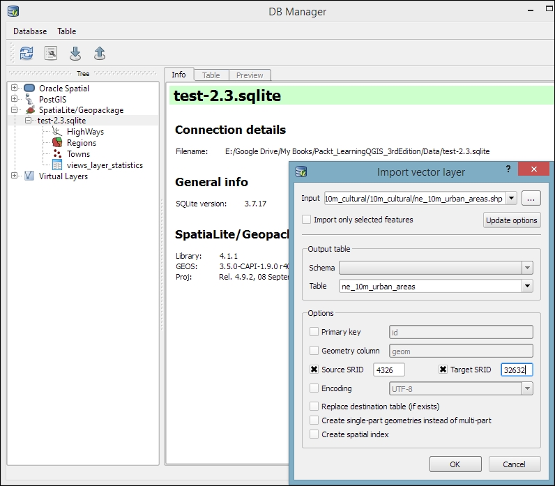
Tip
A handy shortcut for importing data into databases is by directly dragging and dropping files from the main window Browser panel to a database listed in DB Manager. This even works for multiple selected files at once (hold down Ctrl on Windows/Ubuntu or cmd on Mac to select more than one file in the Browser panel). When you drop the files onto the desired database, an Import vector layer dialog will appear, where you can configure the import.
Summary
In this chapter, you learned how to create new layers from scratch. We used a selection of tools to create and edit feature geometries in different ways. Then, we went into editing attributes of single features, feature selections, and whole layers. Next, we reprojected both vector and raster layers, and you learned how to convert between different file formats. We also covered tabular data and how it can be loaded and joined to our spatial data. Furthermore, we explored the use of temporary scratch layers and discussed how to check for topological errors in our data and fix them. We finished this chapter with an example of importing new data into a database.
In the following chapter, we will put our data to good use and see how to perform different kinds of spatial analysis on raster and vector data. We will also take a closer look at the Processing Toolbox, which has made its first appearance in this chapter. You will learn how to use the tools and combine them to create automated workflows.


