Simple example using R neural net library - neuralnet()

Consider a simple dataset of a square of numbers, which will be used to train a neuralnet function in R and then test the accuracy of the built neural network:

INPUT	OUTPUT
0	0
1	1
2	4
3	9
4	16
5	25
6	36
7	49
8	64
9	81
10	100

 

Our objective is to set up the weights and bias so that the model can do what is being done here. The output needs to be modeled on a function of input and the function can be used in future to determine the output based on an input:

######################################################################### 
###Chapter 1 - Introduction to Neural Networks - using R ################ 
###Simple R program to build, train and test neural Networks############# 
######################################################################### 

#Choose the libraries to use
library("neuralnet")

#Set working directory for the training data
setwd("C:/R")
getwd()

#Read the input file
mydata=read.csv('Squares.csv',sep=",",header=TRUE)
mydata
attach(mydata)
names(mydata)

#Train the model based on output from input
model=neuralnet(formula = Output~Input, 
                data = mydata, 
                hidden=10, 
                threshold=0.01 )
print(model)

#Lets plot and see the layers
plot(model)

#Check the data - actual and predicted
final_output=cbind (Input, Output, 
                    as.data.frame(model$net.result) )
colnames(final_output) = c("Input", "Expected Output", 
                           "Neural Net Output" )
print(final_output)
#########################################################################

Let us go through the code line-by-line

To understand all the steps in the code just proposed, we will look at them in detail. Do not worry if a few steps seem unclear at this time, you will be able to look into it in the following examples. First, the code snippet will be shown, and the explanation will follow:

library("neuralnet")

The line in R includes the library neuralnet() in our program. neuralnet() is part of Comprehensive R Archive Network (CRAN), which contains numerous R libraries for various applications.

mydata=read.csv('Squares.csv',sep=",",header=TRUE)
mydata
attach(mydata)
names(mydata)

This reads the CSV file with separator ,(comma), and header is the first line in the file. names() would display the header of the file.

model=neuralnet(formula = Output~Input, 
               data = mydata, 
               hidden=10, 
               threshold=0.01 )

The training of the output with respect to the input happens here. The neuralnet() library is passed the output and input column names (ouput~input), the dataset to be used, the number of neurons in the hidden layer, and the stopping criteria (threshold).

A brief description of the neuralnet package, extracted from the official documentation, is shown in the following table:

neuralnet-package:

Description:

Training of neural networks using the backpropagation, resilient backpropagation with (Riedmiller, 1994) or without weight backtracking (Riedmiller, 1993), or the modified globally convergent version by Anastasiadis et al. (2005). The package allows flexible settings through custom-choice of error and activation function. Furthermore, the calculation of generalized weights (Intrator O & Intrator N, 1993) is implemented.

Details:

Package: neuralnet Type: Package Version: 1.33 Date: 2016-08-05 License: GPL (>=2)

Authors:

Stefan Fritsch, Frauke Guenther (email: [e-mail]) Maintainer: Frauke Guenther (email: [e-mail])

Usage:

neuralnet(formula, data, hidden = 1, threshold = 0.01, stepmax = 1e+05, rep = 1, startweights = NULL, learningrate.limit = NULL, learningrate.factor = list(minus = 0.5, plus = 1.2), learningrate=NULL, lifesign = "none", lifesign.step = 1000, algorithm = "rprop+", err.fct = "sse", act.fct = "logistic", linear.output = TRUE, exclude = NULL,constant.weights = NULL, likelihood = FALSE)

Meaning of the arguments:

formula: A symbolic description of the model to be fitted. data: A dataframe containing the variables specified in formula. hidden: A vector of integers specifying the number of hidden neurons (vertices) in each layer. threshold: A numeric value specifying the threshold for the partial derivatives of the error function as stopping criteria. stepmax: The maximum steps for the training of the neural network. Reaching this maximum leads to a stop of the neural network's training process. rep: The number of repetitions for the neural network's training. startweights: A vector containing starting values for the weights. The weights will not be randomly initialized. learningrate.limit: A vector or a list containing the lowest and highest limit for the learning rate. Used only for RPROP and GRPROP. learningrate.factor: A vector or a list containing the multiplication factors for the upper and lower learning rate, used only for RPROP and GRPROP. learningrate: A numeric value specifying the learning rate used by traditional backpropagation. Used only for traditional backpropagation. lifesign: A string specifying how much the function will print during the calculation of the neural network-'none', 'minimal', or 'full'. lifesign.step: An integer specifying the step size to print the minimal threshold in full lifesign mode. algorithm: A string containing the algorithm type to calculate the neural network. err.fct: A differentiable function that is used for the calculation of the error. act.fct: A differentiable function that is used for smoothing the result of the cross product of the covariate or neurons and the weights. linear.output: Logical. If act.fct should not be applied to the output neurons set linear output to TRUE, otherwise to FALSE. exclude: A vector or a matrix specifying the weights that are excluded from the calculation. constant.weights: A vector specifying the values of the weights that are excluded from the training process and treated as fix. likelihood: Logical. If the error function is equal to the negative log-likelihood function, the information criteria AIC and BIC will be calculated. Furthermore the usage of confidence. interval is meaningful.

 

After giving a brief glimpse into the package documentation, let's review the remaining lines of the proposed code sample:

 print(model)

This command prints the model that has just been generated, as follows:

$result.matrix
                                            1
error                          0.001094100442
reached.threshold              0.009942937680
steps                      34563.000000000000
Intercept.to.1layhid1         12.859227998180
Input.to.1layhid1             -1.267870997079
Intercept.to.1layhid2         11.352189417430
Input.to.1layhid2             -2.185293148851
Intercept.to.1layhid3          9.108325110066
Input.to.1layhid3             -2.242001064132
Intercept.to.1layhid4        -12.895335140784
Input.to.1layhid4              1.334791491801
Intercept.to.1layhid5         -2.764125889399
Input.to.1layhid5              1.037696638808
Intercept.to.1layhid6         -7.891447011323
Input.to.1layhid6              1.168603081208
Intercept.to.1layhid7         -9.305272978434
Input.to.1layhid7              1.183154841948
Intercept.to.1layhid8         -5.056059256828
Input.to.1layhid8              0.939818815422
Intercept.to.1layhid9         -0.716095585596
Input.to.1layhid9             -0.199246231047
Intercept.to.1layhid10        10.041789457410
Input.to.1layhid10            -0.971900813630
Intercept.to.Output           15.279512257145
1layhid.1.to.Output          -10.701406269616
1layhid.2.to.Output           -3.225793088326
1layhid.3.to.Output           -2.935972228783
1layhid.4.to.Output           35.957437333162
1layhid.5.to.Output           16.897986621510
1layhid.6.to.Output           19.159646982676
1layhid.7.to.Output           20.437748965610
1layhid.8.to.Output           16.049490298968
1layhid.9.to.Output           16.328504039013
1layhid.10.to.Output          -4.900353775268

Let's go back to the code analysis:

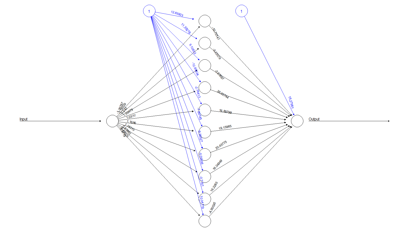
plot(model)

This preceding command plots the neural network for us, as follows:

final_output=cbind (Input, Output, 
                    as.data.frame(model$net.result) )
colnames(final_output) = c("Input", "Expected Output", 
                     "Neural Net Output" )
print(final_output)

This preceding code prints the final output, comparing the output predicted and actual as:

> print(final_output)
 Input Expected Output Neural Net Output
1    0               0     -0.0108685813
2    1               1      1.0277796553
3    2               4      3.9699671691
4    3               9      9.0173879001
5    4              16     15.9950295615
6    5              25     25.0033272826
7    6              36     35.9947137155
8    7              49     49.0046689369
9    8              64     63.9972090104
10   9              81     81.0008391011
11  10             100     99.9997950184