
Chapter 2: Data Cleaning and Pre-processing
Activity 6: Pre-processing using Center and Scale
Solution:
In this exercise, we will perform the center and scale pre-processing operations.
- Load the mlbench library and the PimaIndiansDiabetes dataset:
# Load Library caret
library(caret)
library(mlbench)
# load the dataset PimaIndiansDiabetes
data(PimaIndiansDiabetes)
View the summary:
# view the data
summary(PimaIndiansDiabetes [,1:2])
The output is as follows:
pregnant glucose
Min. : 0.000 Min. : 0.0
1st Qu.: 1.000 1st Qu.: 99.0
Median : 3.000 Median :117.0
Mean : 3.845 Mean :120.9
3rd Qu.: 6.000 3rd Qu.:140.2
Max. :17.000 Max. :199.0
- User preProcess() to pre-process the data to center and scale:
# to standardise we will scale and center
params <- preProcess(PimaIndiansDiabetes [,1:2], method=c("center", "scale"))
- Transform the dataset using predict():
# transform the dataset
new_dataset <- predict(params, PimaIndiansDiabetes [,1:2])
- Print the summary of the new dataset:
# summarize the transformed dataset
summary(new_dataset)
The output is as follows:
pregnant glucose
Min. :-1.1411 Min. :-3.7812
1st Qu.:-0.8443 1st Qu.:-0.6848
Median :-0.2508 Median :-0.1218
Mean : 0.0000 Mean : 0.0000
3rd Qu.: 0.6395 3rd Qu.: 0.6054
Max. : 3.9040 Max. : 2.4429
We will notice that the values are now mean centering values.
Activity 7: Identifying Outliers
Solution:
- Load the dataset:
mtcars = read.csv("mtcars.csv")
- Load the outlier package and use the outlier function to display the outliers:
#Load the outlier library
library(outliers)
- Detect outliers in the dataset using the outlier() function:
#Detect outliers
outlier(mtcars)
The output is as follows:
mpg cyl disp hp drat wt qsec vs am
gear carb
33.900 4.000 472.000 335.000 4.930 5.424 22.900
1.000 1.000 5.000 8.000
- Display the other side of the outlier values:
#This detects outliers from the other side
outlier(mtcars,opposite=TRUE)
The output is as follows:
mpg cyl disp hp drat wt qsec vs am
gear carb
10.400 8.000 71.100 52.000 2.760 1.513 14.500 0.000 0.000
3.000 1.000
- Plot a box plot:
#View the outliers
boxplot(Mushroom)
The output is as follows:
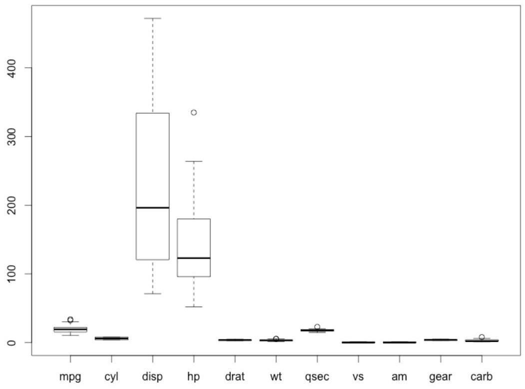
Figure 2.36: Outliers in the mtcars dataset.
The circle marks are the outliers.
Activity 8: Oversampling and Undersampling
Solution:
The detailed solution is as follows:
- Read the mushroom CSV file:
ms<-read.csv('mushrooms.csv')
summary(ms$bruises)
The output is as follows:
f t
4748 3376
- Perform downsampling:
set.seed(9560)
undersampling <- downSample(x = ms[, -ncol(ms)], y = ms$bruises)
table(undersampling$bruises)
The output is as follows:
f t
3376 3376
- Perform oversampling:
set.seed(9560)
oversampling <- upSample(x = ms[, -ncol(ms)],y = ms$bruises)
table(oversampling$bruises)
The output is as follows:
f t
4748 4748
In this activity, we learned to use downSample() and upSample() from the caret package to perform downsampling and oversampling.
Activity 9: Sampling and OverSampling using ROSE
Solution:
The detailed solution is as follows:
- Load the German credit dataset:
#load the dataset
library(caret)
library(ROSE)
data(GermanCredit)
- View the samples in the German credit dataset:
#View samples
head(GermanCredit)
str(GermanCredit)
- Check the number of unbalanced data in the German credit dataset using the summary() method:
#View the imbalanced data
summary(GermanCredit$Class)
The output is as follows:
Bad Good
300 700
- Use ROSE to balance the numbers:
balanced_data <- ROSE(Class ~ ., data = stagec,seed=3)$data
table(balanced_data$Class)
The output is as follows:
Good Bad
480 520
Using the preceding example, we learned how to increase and decrease the class count using ROSE.