Plotting curves from file data

As explained earlier, matplotlib only handles plotting. If you want to plot data stored in a file, you will have to use Python code to read the file and extract the data you need.

How to do it...

Let's assume that we have time series stored in a plain text file named my_data.txt as follows:

0  0
1  1
2  4
4 16
5 25
6 36

A minimalistic pure Python approach to read and plot that data would go as follows:

import matplotlib.pyplot as plt

X, Y = [], []
for line in open('my_data.txt', 'r'):
  values = [float(s) for s in line.split()]
  X.append(values[0])
  Y.append(values[1])

plt.plot(X, Y)
plt.show()

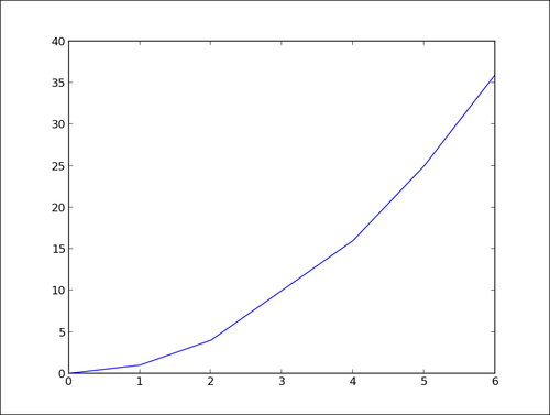
This script, together with the data stored in my_data.txt, will produce the following graph:

How it works...

The following are some explanations on how the preceding script works:

• The line X, Y = [], [] initializes the list of coordinates X and Y as empty lists.

• The line for line in open('my_data.txt', 'r') defines a loop that will iterate each line of the text file my_data.txt. On each iteration, the current line extracted from the text file is stored as a string in the variable line.

• The line values = [float(s) for s in line.split()] splits the current line around empty characters to form a string of tokens. Those tokens are then interpreted as floating point values. Those values are stored in the list values.

• Then, in the two next lines, X.append(values[0]) and Y.append(values[1]), the values stored in values are appended to the lists X and Y.

The following equivalent one-liner to read a text file may bring a smile to those more familiar with Python:

import matplotlib.pyplot as plt

with open('my_data.txt', 'r') as f:
  X, Y = zip(*[[float(s) for s in line.split()] for line in f])

plt.plot(X, Y)
plt.show()

There's more...

In our data loading code, note that there is no serious checking or error handling going on. In any case, one might remember that a good programmer is a lazy programmer. Indeed, since NumPy is so often used with matplotlib, why not use it here? Run the following script to enable NumPy:

import numpy as np
import matplotlib.pyplot as plt

data = np.loadtxt('my_data.txt')

plt.plot(data[:,0], data[:,1])
plt.show()

This is as short as the one-liner shown in the preceding section, yet easier to read, and it will handle many error cases that our pure Python code does not handle. The following point describes the preceding script:

• The numpy.loadtxt() function reads a text file and returns a 2D array. With NumPy, 2D arrays are not a list of lists, they are true, full-blown matrices.

• The variable data is a NumPy 2D array, which give us the benefit of being able to manipulate rows and columns of a matrix as a 1D array. Indeed, in the line plt.plot(data[:,0], data[:,1]), we give the first column of data as x coordinates and the second column of data as y coordinates. This notation is specific to NumPy.

Along with making the code shorter and simpler, using NumPy brings additional advantages. For large files, using NumPy will be noticeably faster (the NumPy module is mostly written in C), and storing the whole dataset as a NumPy array can save memory as well. Finally, using NumPy allows you to support other common file formats (CVS and Matlab) for numerical data without much effort.

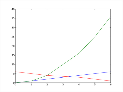
As a way to demonstrate all that we have seen so far, let's consider the following task. A file contains N columns of values, describing N–1 curves. The first column contains the x coordinates, the second column contains the y coordinates of the first curve, the third column contains the y coordinates of the second curve, and so on. We want to display those N–1 curves. We will do so by using the following code:

import numpy as np
import matplotlib.pyplot as plt

data = np.loadtxt('my_data.txt')
for column in data.T:
  plt.plot(data[:,0], column)

plt.show()

The file my_data.txt should contain the following content:

0 0 6
1 1 5
2 4 4
4 16 3
5 25 2
6 36 1

Then we get the following graph:

We did the job with little effort by exploiting two tricks. In NumPy notation, data.T is a transposed view of the 2D array data—rows are seen as columns and columns are seen as rows. Also, we can iterate over the rows of a multidimensional array by doing for row in data. Thus, doing for column in data.T will iterate over the columns of an array. With a few lines of code, we have a fairly general plotting generic script.