Search icon CANCEL
Subscription
0
Cart icon
Your Cart (0 item)
Close icon
You have no products in your basket yet
Arrow left icon
Explore Products
Best Sellers
New Releases
Books
Videos
Audiobooks
Learning Hub
Conferences
Free Learning
Arrow right icon
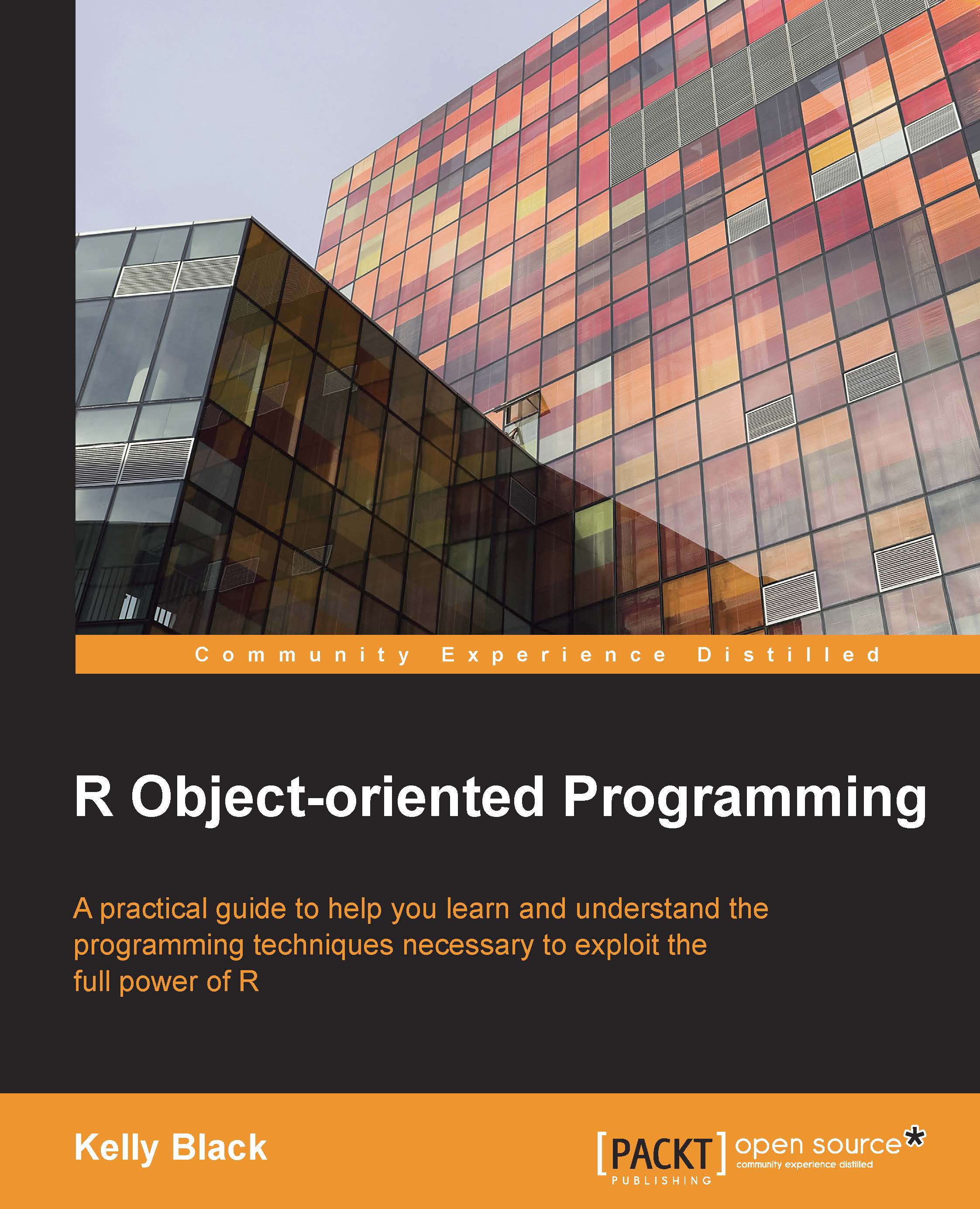
R Object-oriented Programming

R Object-oriented Programming: A practical guide to help you learn and understand the programming techniques necessary to exploit the full power of R

eBook
$9.99 $28.99
Paperback
$48.99
Subscription
Free Trial
Renews at $19.99p/m

What do you get with a Packt Subscription?

Free for first 7 days. $19.99 p/m after that. Cancel any time!
Product feature icon Unlimited ad-free access to the largest independent learning library in tech. Access this title and thousands more!
Product feature icon 50+ new titles added per month, including many first-to-market concepts and exclusive early access to books as they are being written.
Product feature icon Innovative learning tools, including AI book assistants, code context explainers, and text-to-speech.
Product feature icon Thousands of reference materials covering every tech concept you need to stay up to date.
Subscribe now
View plans & pricing
Table of content icon View table of contents Preview book icon Preview Book

R Object-oriented Programming

Chapter 1. Data Types

In this chapter, we provide a broad overview of the different data types available in the R environment. This material is introductory in nature, and this chapter ensures that important information on implementing algorithms is available to you. There are roughly five parts in this chapter:

  • Working with variables in the R environment: This section gives you a broad overview of interacting with the R shell, creating variables, deleting variables, saving variables, and loading variables
  • Discrete data types: This section gives you an overview of the principle data types used to represent discrete data
  • Continuous data types: This section gives you an overview of the principle data types used to represent continuous data
  • Introduction to vectors: This section gives you an introduction to vectors and manipulating vectors in R
  • Special data types: This section gives you a list of other data types that do not fit in the other categories or have other meanings

Assignment

The R environment is an interactive shell. Commands are entered using the keyboard, and the environment should feel familiar to anyone used to MATLAB or the Python interactive interpreter. To assign a value to a variable, you can usually use the = symbol in the same way as these other interpreters. The difference with R, however, is that there are other ways to assign a variable, and their behavior depends on the context.

Another way to assign a value to a variable is to use the <- symbols (sometimes called operators). At first glance, it seems odd to have different ways to assign a value, but we will see that variables can be saved in different environments. The same name may be used in different environments, and the name can be ambiguous. We will adopt the use of the <- operator in this text because it is the most common operator, and it is also the least likely to cause confusion in different contexts.

The R environment manages memory and variable names dynamically. To create a new variable, simply assign a value to it, as follows:

> a <- 6
> a
[1] 6

A variable has a scope, and the meaning of a variable name can vary depending on the context. For example, if you refer to a variable within a function (think subroutine) or after attaching a dataset, then there may be multiple variables in the workspace with the same name. The R environment maintains a search path to determine which variable to use, and we will discuss these details as they arise.

The <- operator for the assignment will work in any context while the = operator only works for complete expressions. Another option is to use the <<- operator. The advantage of the <<- operator is that it instructs the R environment to search parent environments to see whether the variable already exists. In some contexts, within a function for example, the <- operator will create a new variable; however, the <<- operator will make use of an existing variable outside of the function if it is found.

Another way to assign variables is to use the -> and ->> operators. These operators are similar to those given previously. The only difference is that they reverse the direction of assignment, as follows:

> 14.5 -> a
> 1/12.0 ->> b
> a
[1] 14.5
> b
[1] 0.08333333

The workspace

The R environment keeps track of variables as well as allocates and manages memory as it is requested. One command to list the currently defined variables is the ls command. A variable can be deleted using the rm command. In the following example, the a and b variables have been changed, and the a variable is deleted:

> a <-  17.5
> b <- 99/4
> ls()
[1] "a" "b"
> objects()
[1] "a" "b"
> rm(a)
> ls()
[1] "b"

If you wish to delete all of the variables in the workspace, the list option in the rm command can be combined with the ls command, as follows:

> ls()
[1] "b"
> rm(list=ls())
> ls()
character(0)

A wide variety of other options are available. For example, there are directory options to show and set the current directory, as follows:

> getwd()
[1] "/home/black"
> setwd("/tmp")
> getwd()
[1] "/tmp"
> dir()
 [1] "antActivity.R"             "betterS3.R"               
 [3] "chiSquaredArea.R"          "firstS3.R"                
[5] "math100.csv"               "opsTesting.R"             
[7] "probabilityExampleOne.png" "s3.R"                      
[9] "s4Example.R"

Another important task is to save and load a workspace. The save and save.image commands can be used to save the current workspace. The save command allows you to save a particular variable, and the save.image command allows you to save the entire workspace. The usage of these commands is as follows:

> save(a,file="a.RData")
> save.image("wholeworkspace.Rdata")

These commands have a variety of options. For example, the ascii option is a commonly used option to ensure that the data file is in a (nearly) human-readable form. The help command can be used to get more details and see more of the options that are available. In the following example, the variable a is saved in a file, a.RData, and the file is saved in a human-readable format:

> save(a,file="a.RData",ascii=TRUE)
> save.image(" wholeworkspace.RData",ascii=TRUE)
> help(save)

As an alternative to the help command, the ? operator can also be used to get the help page for a given command. An additional command is the help.search command that is used to search the help files for a given string. The ?? operator is also available to perform a search for a given string.

The information in a file can be read back into the workspace using the load command:

> load("a.RData")
> ls()
[1] "a"
> a
[1] 19

Another question that arises with respect to a variable is how it is stored. The two commands to determine this are mode and storage.mode. You should try to use these commands for each of the data types described in the following subsections. Basically, these commands can make it easier to determine whether a variable is a numeric value or another basic data type.

The previous commands provide options for saving the values of the variables within a workspace. They do not save the commands that you have entered. These commands are referred to as the history within the R workspace, and you can save your history using the savehistory command. The history can be displayed using the history command, and the loadhistory command can be used to replay the commands in a file.

The last command given here is the command to quit, q(). Some people consider this to be the most important command because without it you would never be able to leave R. The rest of us are not sure why it is necessary.

Discrete data types

One of the features of the R environment is the rich collection of data types that are available. Here, we briefly list some of the built-in data types that describe discrete data. The four data types discussed are the integer, logical, character, and factor data types. We also introduce the idea of a vector, which is the default data structure for any variable. A list of the commands discussed here is given in Table 2 and Table 3.

It should be noted that the default data type in R, for a number, is a double precision number. Strings can be interpreted in a variety of ways, usually as either a string or a factor. You should be careful to make sure that R is storing information in the format that you want, and it is important to double-check this important aspect of how data is tracked.

Integer

The first discrete data type examined is the integer type. Values are 32-bit integers. In most circumstances, a number must be explicitly cast as being an integer, as the default type in R is a double precision number. There are a variety of commands used to cast integers as well as allocate space for integers. The integer command takes a number for an argument and will return a vector of integers whose length is given by the argument:

> bubba <- integer(12)
> bubba
 [1] 0 0 0 0 0 0 0 0 0 0 0 0
> bubba[1]
[1] 0
> bubba[2]
[1] 0
> bubba[[4]]
[1] 0
>  b[4] <- 15
> b
 [1]  0  0  0 15  0  0  0  0  0  0  0  0

In the preceding example, a vector of twelve integers was defined. The default values are zero, and the individual entries in the vector are accessed using braces. The first entry in the vector has index 1, so in this example, bubba[1] refers to the initial entry in the vector. Note that there are two ways to access an element in the vector: single versus double braces. For a vector, the two methods are nearly the same, but when we explore the use of lists as opposed to vectors, the meaning will change. In short, the double braces return objects of the same type as the elements within the vector, and the single braces return values of the same type as the variable itself. For example, using single braces on a list will return a list, while double braces may return a vector.

A number can be cast as an integer using the as.integer command. A variable's type can be checked using the typeof command. The typeof command indicates how R stores the object and is different from the class command, which is an attribute that you can change or query:

> as.integer(13.2)
[1] 13
> thisNumber <- as.integer(8/3)
> typeof(thisNumber)
[1] "integer"

Note that a sequence of numbers can be automatically created using either the : operator or the seq command:

> 1:5
[1] 1 2 3 4 5
> myNum <- as.integer(1:5)


> myNum[1]
[1] 1
> myNum[3]
[1] 3

> seq(4,11,by=2)
[1]  4  6  8 10
> otherNums <- seq(4,11,by=2)


> otherNums[3]
[1] 8

A common task is to determine whether or not a variable is of a certain type. For integers, the is.integer command is used to determine whether or not a variable has an integer type:

> a <- 1.2
> typeof(a)
[1] "double"
> is.integer(a)
[1] FALSE

> a <- as.integer(1.2)
> typeof(a)
[1] "integer"
> is.integer(a)
[1] TRUE

Logical

Logical data consists of variables that are either true or false. The words TRUE and FALSE are used to designate the two possible values of a logical variable. (The TRUE value can also be abbreviated to T, and the FALSE value can be abbreviated to F.) The basic commands associated with logical variables are similar to the commands for integers discussed in the previous subsection. The logical command is used to allocate a vector of Boolean values. In the following example, a logical vector of length 10 is created. The default value is FALSE, and the Boolean not operator is used to flip the values to evaluate to TRUE:

> b <- logical(10)
> b
 [1] FALSE FALSE FALSE FALSE FALSE FALSE FALSE FALSE FALSE FALSE
> b[3]
[1] FALSE
> !b
 [1] TRUE TRUE TRUE TRUE TRUE TRUE TRUE TRUE TRUE TRUE
> !b[5]
[1] TRUE
> typeof(b)
[1] "logical"
> mode(b)
[1] "logical"
> storage.mode(b)
[1] "logical"
>  b[3] <- TRUE
> b
 [1] FALSE FALSE  TRUE FALSE FALSE FALSE FALSE FALSE FALSE FALSE

To cast a value to a logical type, you can use the as.logical command. Note that zero is mapped to a value of FALSE and other numbers are mapped to a value of TRUE:

> a <- -1:1
> a
[1] -1  0  1
> as.logical(a)
[1]  TRUE FALSE  TRUE

To determine whether or not a value has a logical type, you use the is.logical command:

> b <- logical(4)
> b
[1] FALSE FALSE FALSE FALSE
> is.logical(b)
[1] TRUE

The standard operators for logical operations are available, and a list of some of the more common operations is given in Table 1. Note that there is a difference between operations such as & and &&. A single & is used to perform an and operation on each pairwise element of two vectors, while the double && returns a single logical result using only the first elements of the vectors:

> l1 <- c(TRUE,FALSE)
> l2 <- c(TRUE,TRUE)
> l1&l1
[1]  TRUE FALSE
> l1&&l1
[1] TRUE
> l1|l2
[1] TRUE TRUE
> l1||l2
[1] TRUE

Tip

You can download the example code files for all Packt books you have purchased from your account at http://www.packtpub.com. An additional source for the examples in this book can be found at https://github.com/KellyBlack/R-Object-Oriented-Programming. If you purchased this book elsewhere, you can visit http://www.packtpub.com/support and register to have the files e-mailed directly to you.

The following table shows various logical operators and their description:

Logical Operator

Description

<

Less than

>

Greater that

<=

Less than or equal to

>=

Greater than or equal to

==

Equal to

!=

Not equal to

|

Entrywise or

||

Or

!

Not

&

Entrywise and

&&

And

xor(a,b)

Exclusive or

Table 1 – list of operators for logical variables

Character

One common way to store information is to save data as characters or strings. Character data is defined using either single or double quotes:

> a <- "hello"
> a
[1] "hello"
> b <- 'there'
> b
[1] "there"
> typeof(a)
[1] "character"

The character command can be used to allocate a vector of character-valued strings, as follows:

> many <- character(3)
> many
[1] "" "" ""
> many[2] <- "this is the second"
> many[3] <- 'yo, third!'
> many[1] <- "and the first"
> many
[1] "and the first"      "this is the second" "yo, third!"        

A value can be cast as a character using the as.character command, as follows:

> a <- 3.0
> a
[1] 3
> b <- as.character(a)
> b
[1] "3"

Finally, the is.character command takes a single argument, and it returns a value of TRUE if the argument is a string:

> a <- as.character(4.5)
> a
[1] "4.5"
> is.character(a)
[1] TRUE

Factors

Another common way to record data is to provide a discrete set of levels. For example, the results of an individual trial in an experiment may be denoted by a value of a, b, or c. Ordinal data of this kind is referred to as a factor in R. The commands and ideas are roughly parallel to the data types described previously. There are some subtle differences with factors, though. Factors are used to designate different levels and can be considered ordered or unordered. There are a large number of options, and it is wise to consult the help pages for factors using the (help(factor)) command. One thing to note, though, is that the typeof command for a factor will return an integer.

Factors can be defined using the factor command, as follows:

> lev <- factor(x=c("one","two","three","one"))
> lev
[1] one   two   three one  
Levels: one three two
> levels(lev)
[1] "one"   "three" "two"  
> sort(lev)
[1] one   one   two   three
Levels: one two three

>  lev <- factor(x=c("one","two","three","one"),levels=c("one","two","three"))
> lev
[1] one   two   three one  
Levels: one two three
> levels(lev)
[1] "one"   "two"   "three"
> sort(lev)
[1] one   one   two   three
Levels: one two three

The techniques used to cast a variable to a factor or test whether a variable is a factor are similar to the previous examples. A variable can be cast as a factor using the as.factor command. Also, the is.factor command can be used to determine whether or not a variable has a type of factor.

Continuous data types

The data types for continuous data types are given here. The double and complex data types are given. A list of the commands discussed here is given in Table 2 and Table 3.

Double

The default numeric data type in R is a double precision number. The commands are similar to those of the integer data type discussed previously. The double command can be used to allocate a vector of double precision numbers, and the numbers within the vector are accessed using braces:

> d <- double(8)
> d
[1] 0 0 0 0 0 0 0 0
> typeof(d)
[1] "double"
> d[3] <- 17
> d
[1]  0  0 17  0  0  0  0  0

The techniques used to cast a variable to a double precision number and test whether a variable is a double precision number are similar to the examples seen previously. A variable can be cast as a double precision number using the as.double command. Also, to determine whether a variable is a double precision number, the as.double command can be used.

Complex

Arithmetic for complex numbers is supported in R, and most math functions will react properly when given a complex number. You can append i to the end of a number to force it to be the imaginary part of a complex number, as follows:

> 1i
[1] 0+1i
> 1i*1i
[1] -1+0i
> z <- 3+2i
> z
[1] 3+2i
> z*z
[1] 5+12i
> Mod(z)
[1] 3.605551
> Re(z)
[1] 3
> Im(z)
[1] 2
> Arg(z)
[1] 0.5880026
> Conj(z)
[1] 3-2i

The complex command can also be used to define a vector of complex numbers. There are a number of options for the complex command, so a quick check of the help page, (help(complex)), is recommended:

> z <- complex(3)
> z
[1] 0+0i 0+0i 0+0i
> typeof(z)
[1] "complex"
> z <- complex(real=c(1,2),imag=c(3,4))
> z
[1] 1+3i 2+4i
> Re(z)
[1] 1 2

The techniques to cast a variable to a complex number and to test whether or not a variable is a complex number are similar to the methods seen previously. A variable can be cast as complex using the as.complex command. Also, to test whether or not a variable is a complex number, the as.complex command can be used.

Special data types

There are two other common data types that occur that are important. We will discuss these two data types and provide a note about objects. The two data types are NA and NULL. These are brief comments, as these are recurring topics that we will revisit many times.

The first data type is a constant, NA. This is a type used to indicate a missing value. It is a constant in R, and a variable can be tested using the is.na command, as follows:

> n <- c(NA,2,3,NA,5)
> n
[1] NA  2  3 NA  5
> is.na(n)
[1]  TRUE FALSE FALSE  TRUE FALSE
> n[!is.na(n)]
[1] 2 3 5

Another special type is the NULL type. It has the same meaning as the null keyword in the C language. It is not an actual type but is used to determine whether or not an object exists:

> a <- NULL
> typeof(a)
[1] "NULL"

Finally, we'll quickly explore the term objects. The variables that we defined in all of the preceding examples are treated as objects within the R environment. When we start writing functions and creating classes, it will be important to realize that they are treated like variables. The names used to assign variables are just a shortcut for R to determine where an object is located.

For example, the complex command is used to allocate a vector of complex values. The command is defined to be a set of instructions, and there is an object called complex that points to those instructions:

> complex
function (length.out = 0L, real = numeric(), imaginary = numeric(),
    modulus = 1, argument = 0)
{
    if (missing(modulus) && missing(argument)) {
        .Internal(complex(length.out, real, imaginary))
    }
    else {
        n <- max(length.out, length(argument), length(modulus))
        rep_len(modulus, n) * exp((0+1i) * rep_len(argument,
            n))
    }
}
<bytecode: 0x2489c80>
<environment: namespace:base>

There is a difference between calling the complex()function and referring to the set of instructions located at complex.

Notes on the as and is functions

Two common tasks are to determine whether a variable is of a given type and to cast a variable to different types. The commands to determine whether a variable is of a given type generally start with the is prefix, and the commands to cast a variable to a different type generally start with the as prefix. The list of commands to determine whether a variable is of a given type are given in the following table:

Type to check

Command

Integer

is.integer

Logical

is.logical

Character

is.character

Factor

is.factor

Double

is.double

Complex

is.complex

NA

is.NA

List

is.list

Table 2 – commands to determine whether a variable is of a particular type

The commands used to cast a variable to a different type are given in Table 3. These commands take a single argument and return a variable of the given type. For example, the as.character command can be used to convert a number to a string.

The commands in the previous table are used to test what type a variable has. The following table provides the commands that are used to change a variable of one type to another type:

Type to convert to

Command

Integer

as.integer

Logical

as.logical

Character

as.character

Factor

as.factor

Double

as.double

Complex

as.complex

NA

as.NA

List

as.list

Table 3 – commands to cast a variable into a particular type

Summary

In this chapter, we examined some of the data types available in the R environment. These include discrete data types such as integers and factors. It also includes continuous data types such as real and complex data types. We also examined ways to test a variable to determine what type it is.

In the next chapter, we look at the data structures that can be used to keep track of data. This includes vectors and data types such as lists and data frames that can be constructed from vectors.

Left arrow icon Right arrow icon

Description

This book is designed for people with some experience in basic programming practices. It is also assumed that they have some basic experience using R and are familiar using the command line in an R environment. Our primary goal is to raise a beginner to a more advanced level to make him/her more comfortable creating programs and extending R to solve common problems.

What you will learn

  • Understand the fundamental data types and data structures in R
  • Explore the basic commands and tools to aid in addressing common tasks
  • Use the primary control structures in R to implement algorithms
  • Use and develop S3 and S4 classes
  • Discover the differences between S3 and S4 classes
  • Bring different ideas together to solve common problems
  • Understand the fundamental design and approach to objectoriented programming in R

Product Details

Country selected
Publication date, Length, Edition, Language, ISBN-13
Publication date : Oct 27, 2014
Length: 190 pages
Edition : 1st
Language : English
ISBN-13 : 9781783986682
Category :
Languages :

What do you get with a Packt Subscription?

Free for first 7 days. $19.99 p/m after that. Cancel any time!
Product feature icon Unlimited ad-free access to the largest independent learning library in tech. Access this title and thousands more!
Product feature icon 50+ new titles added per month, including many first-to-market concepts and exclusive early access to books as they are being written.
Product feature icon Innovative learning tools, including AI book assistants, code context explainers, and text-to-speech.
Product feature icon Thousands of reference materials covering every tech concept you need to stay up to date.
Subscribe now
View plans & pricing

Product Details

Publication date : Oct 27, 2014
Length: 190 pages
Edition : 1st
Language : English
ISBN-13 : 9781783986682
Category :
Languages :

Packt Subscriptions

See our plans and pricing
Modal Close icon
$19.99 billed monthly
Feature tick icon Unlimited access to Packt's library of 7,000+ practical books and videos
Feature tick icon Constantly refreshed with 50+ new titles a month
Feature tick icon Exclusive Early access to books as they're written
Feature tick icon Solve problems while you work with advanced search and reference features
Feature tick icon Offline reading on the mobile app
Feature tick icon Simple pricing, no contract
$199.99 billed annually
Feature tick icon Unlimited access to Packt's library of 7,000+ practical books and videos
Feature tick icon Constantly refreshed with 50+ new titles a month
Feature tick icon Exclusive Early access to books as they're written
Feature tick icon Solve problems while you work with advanced search and reference features
Feature tick icon Offline reading on the mobile app
Feature tick icon Choose a DRM-free eBook or Video every month to keep
Feature tick icon PLUS own as many other DRM-free eBooks or Videos as you like for just $5 each
Feature tick icon Exclusive print discounts
$279.99 billed in 18 months
Feature tick icon Unlimited access to Packt's library of 7,000+ practical books and videos
Feature tick icon Constantly refreshed with 50+ new titles a month
Feature tick icon Exclusive Early access to books as they're written
Feature tick icon Solve problems while you work with advanced search and reference features
Feature tick icon Offline reading on the mobile app
Feature tick icon Choose a DRM-free eBook or Video every month to keep
Feature tick icon PLUS own as many other DRM-free eBooks or Videos as you like for just $5 each
Feature tick icon Exclusive print discounts

Frequently bought together


Stars icon
Total $ 158.97
R for Data Science
$54.99
Learning R for Geospatial Analysis
$54.99
R Object-oriented Programming
$48.99
Total $ 158.97 Stars icon
Banner background image

Table of Contents

13 Chapters
1. Data Types Chevron down icon Chevron up icon
2. Organizing Data Chevron down icon Chevron up icon
3. Saving Data and Printing Results Chevron down icon Chevron up icon
4. Calculating Probabilities and Random Numbers Chevron down icon Chevron up icon
5. Character and String Operations Chevron down icon Chevron up icon
6. Converting and Defining Time Variables Chevron down icon Chevron up icon
7. Basic Programming Chevron down icon Chevron up icon
8. S3 Classes Chevron down icon Chevron up icon
9. S4 Classes Chevron down icon Chevron up icon
10. Case Study – Course Grades Chevron down icon Chevron up icon
11. Case Study – Simulation Chevron down icon Chevron up icon
A. Package Management Chevron down icon Chevron up icon
Index Chevron down icon Chevron up icon

Customer reviews

Top Reviews
Rating distribution
Full star icon Full star icon Full star icon Full star icon Half star icon 4.4
(9 Ratings)
5 star 66.7%
4 star 22.2%
3 star 0%
2 star 11.1%
1 star 0%
Filter icon Filter
Top Reviews

Filter reviews by


Harold Henson Sep 13, 2021
Full star icon Full star icon Full star icon Full star icon Full star icon 5
I learned object oriented programming with C++ and love the Python 3.0 paradigm. However, as an econometrician most of the demand for my work is in the R, so a shift was inevitable. It is surprising how different the R conceptual framework is from C++. This book make it seem natural and even made sense.
Amazon Verified review Amazon
fabio veronesi Nov 28, 2014
Full star icon Full star icon Full star icon Full star icon Full star icon 5
Overall, I think this book does a good of providing the reader with a strong and neat introduction to all the bits of coding required to become more comfortable writing advance scripts. It covers aspects of the R language that are often overlooked by introductory books.For example, it provides an extensive overview with two well written examples on the use of S3 and S4 classes. In the examples, the reader uses all the programming skills learning from the book to produce R programs to solve very practical task, such as grade students and performing a Monte Carlo simulation. In these programs the reader will add functions and methods to read files and perform statistical analysis, while creating R programs that can easily be shared with other users.Another aspect that I found interesting it the focus on web data. Nowadays lots of data are gathered from the web directly or using APIs. This book provides a good introduction to read, write and manipulate such data and therefore I think it is potentially very useful for the future generations of R users.The book is targeted to post-beginners, therefore people already familiar with R or at least familiar with other object-oriented programming languages. However, I think such a book is very good value for money because it is structure in such a way that it become very easy to look-up functions and commands that maybe we do not use every day and therefore we forgot how to use. I think I will consult this book on a regular basis for my work!For my full review please look at: http://r-video-tutorial.blogspot.com/2014/11/r-object-oriented-programming-book.html
Amazon Verified review Amazon
Arnold Salvacion Dec 01, 2014
Full star icon Full star icon Full star icon Full star icon Full star icon 5
Recently, Packt Publishing publish the book R Object-oriented Programming. The eleven chapter book covers from basic data types in R to a more advanced method such as simulation and writing functions. Different data types (i.e. integer, character, factor) are discussed in-depth in the book as well as numeric and string operations. The good thing with it is that it walks the reader from simple to complicated topic making it easier to learn the language. There are two chapters dedicated in discussing about S3 and S4 classes which are not commonly found published books about R. The last two chapters of the book are dedicated case studies wherein the reader can apply all the learnings from previous chapter. A very good book for beginners and basic users who want to advance their skill and explore the full potential of R as a programming language. Good book to have!
Amazon Verified review Amazon
Ketan Feb 03, 2015
Full star icon Full star icon Full star icon Full star icon Full star icon 5
R Object Oriented Programming is an excellent book to understand the fundamental data types and data structures in R. It investigates the fundamental commands and tools to aid in dealing with common tasks. It helps comprehend the primary blueprint and approach to object-oriented programming in R
Amazon Verified review Amazon
Adrian Thompson Dec 24, 2014
Full star icon Full star icon Full star icon Full star icon Full star icon 5
Only read two chapters so far, covered the basics, it's looking good. Delivery was quick and was well packaged A++ Seller
Amazon Verified review Amazon
Get free access to Packt library with over 7500+ books and video courses for 7 days!
Start Free Trial

FAQs

What is included in a Packt subscription? Chevron down icon Chevron up icon

A subscription provides you with full access to view all Packt and licnesed content online, this includes exclusive access to Early Access titles. Depending on the tier chosen you can also earn credits and discounts to use for owning content

How can I cancel my subscription? Chevron down icon Chevron up icon

To cancel your subscription with us simply go to the account page - found in the top right of the page or at https://subscription.packtpub.com/my-account/subscription - From here you will see the ‘cancel subscription’ button in the grey box with your subscription information in.

What are credits? Chevron down icon Chevron up icon

Credits can be earned from reading 40 section of any title within the payment cycle - a month starting from the day of subscription payment. You also earn a Credit every month if you subscribe to our annual or 18 month plans. Credits can be used to buy books DRM free, the same way that you would pay for a book. Your credits can be found in the subscription homepage - subscription.packtpub.com - clicking on ‘the my’ library dropdown and selecting ‘credits’.

What happens if an Early Access Course is cancelled? Chevron down icon Chevron up icon

Projects are rarely cancelled, but sometimes it's unavoidable. If an Early Access course is cancelled or excessively delayed, you can exchange your purchase for another course. For further details, please contact us here.

Where can I send feedback about an Early Access title? Chevron down icon Chevron up icon

If you have any feedback about the product you're reading, or Early Access in general, then please fill out a contact form here and we'll make sure the feedback gets to the right team. 

Can I download the code files for Early Access titles? Chevron down icon Chevron up icon

We try to ensure that all books in Early Access have code available to use, download, and fork on GitHub. This helps us be more agile in the development of the book, and helps keep the often changing code base of new versions and new technologies as up to date as possible. Unfortunately, however, there will be rare cases when it is not possible for us to have downloadable code samples available until publication.

When we publish the book, the code files will also be available to download from the Packt website.

How accurate is the publication date? Chevron down icon Chevron up icon

The publication date is as accurate as we can be at any point in the project. Unfortunately, delays can happen. Often those delays are out of our control, such as changes to the technology code base or delays in the tech release. We do our best to give you an accurate estimate of the publication date at any given time, and as more chapters are delivered, the more accurate the delivery date will become.

How will I know when new chapters are ready? Chevron down icon Chevron up icon

We'll let you know every time there has been an update to a course that you've bought in Early Access. You'll get an email to let you know there has been a new chapter, or a change to a previous chapter. The new chapters are automatically added to your account, so you can also check back there any time you're ready and download or read them online.

I am a Packt subscriber, do I get Early Access? Chevron down icon Chevron up icon

Yes, all Early Access content is fully available through your subscription. You will need to have a paid for or active trial subscription in order to access all titles.

How is Early Access delivered? Chevron down icon Chevron up icon

Early Access is currently only available as a PDF or through our online reader. As we make changes or add new chapters, the files in your Packt account will be updated so you can download them again or view them online immediately.

How do I buy Early Access content? Chevron down icon Chevron up icon

Early Access is a way of us getting our content to you quicker, but the method of buying the Early Access course is still the same. Just find the course you want to buy, go through the check-out steps, and you’ll get a confirmation email from us with information and a link to the relevant Early Access courses.

What is Early Access? Chevron down icon Chevron up icon

Keeping up to date with the latest technology is difficult; new versions, new frameworks, new techniques. This feature gives you a head-start to our content, as it's being created. With Early Access you'll receive each chapter as it's written, and get regular updates throughout the product's development, as well as the final course as soon as it's ready.We created Early Access as a means of giving you the information you need, as soon as it's available. As we go through the process of developing a course, 99% of it can be ready but we can't publish until that last 1% falls in to place. Early Access helps to unlock the potential of our content early, to help you start your learning when you need it most. You not only get access to every chapter as it's delivered, edited, and updated, but you'll also get the finalized, DRM-free product to download in any format you want when it's published. As a member of Packt, you'll also be eligible for our exclusive offers, including a free course every day, and discounts on new and popular titles.