Search icon CANCEL
Subscription
0
Cart icon
Your Cart (0 item)
Close icon
You have no products in your basket yet
Save more on your purchases! discount-offer-chevron-icon
Savings automatically calculated. No voucher code required.
Arrow left icon
Explore Products
Best Sellers
New Releases
Books
Videos
Audiobooks
Learning Hub
Newsletter Hub
Free Learning
Arrow right icon
timer SALE ENDS IN
0 Days
:
00 Hours
:
00 Minutes
:
00 Seconds
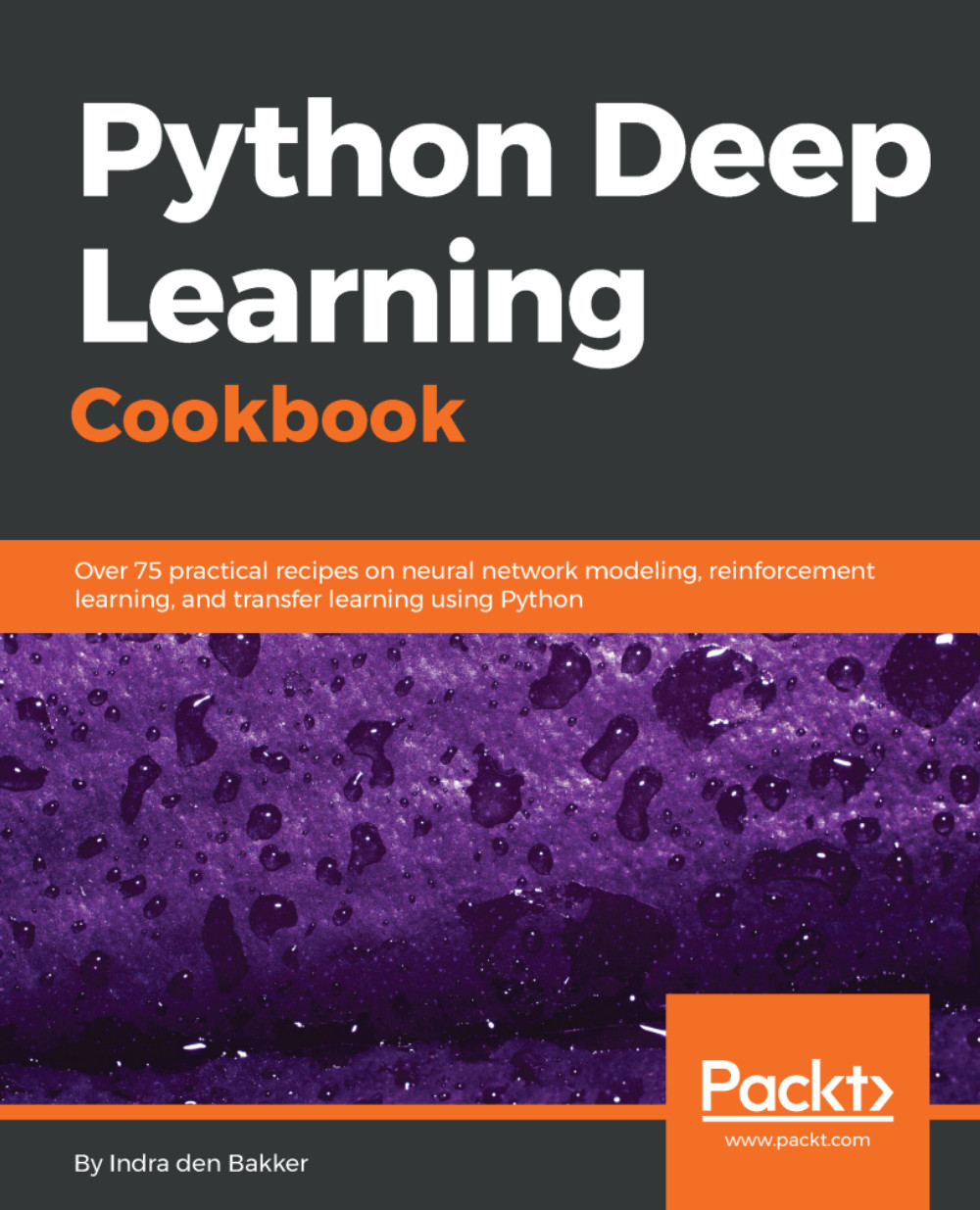
Python Deep Learning Cookbook

Python Deep Learning Cookbook: Over 75 practical recipes on neural network modeling, reinforcement learning, and transfer learning using Python

eBook
$9.99 $39.99
Paperback
$48.99
Subscription
Free Trial
Renews at $19.99p/m

What do you get with Print?

Product feature icon Instant access to your digital eBook copy whilst your Print order is Shipped
Product feature icon Paperback book shipped to your preferred address
Product feature icon Download this book in EPUB and PDF formats
Product feature icon Access this title in our online reader with advanced features
Product feature icon DRM FREE - Read whenever, wherever and however you want
OR
Modal Close icon
Payment Processing...
tick Completed

Shipping Address

Billing Address

Shipping Methods
Table of content icon View table of contents Preview book icon Preview Book

Python Deep Learning Cookbook

Programming Environments, GPU Computing, Cloud Solutions, and Deep Learning Frameworks

This chapter focuses on technical solutions to set up popular deep learning frameworks. First, we provide solutions to set up a stable and flexible environment on local machines and with cloud solutions. Next, all popular Python deep learning frameworks are discussed in detail:

  • Setting up a deep learning environment
  • Launching an instance on Amazon Web Services (AWS)
  • Launching an instance on Google Cloud Platform (GCP)
  • Installing CUDA and cuDNN
  • Installing Anaconda and libraries
  • Connecting with Jupyter Notebook on a server
  • Building state-of-the-art, production-ready models with TensorFlow
  • Intuitively building networks with Keras
  • Using PyTorch's dynamic computation graphs for RNNs
  • Implementing high-performance models with CNTK
  • Building efficient models with MXNet
  • Defining networks using simple and efficient code with Gluon

Introduction

The recent advancements in deep learning can be, to some extent, attributed to the advancements in computing power. The increase in computing power, more specifically the use of GPUs for processing data, has contributed to the leap from shallow neural networks to deeper neural networks. In this chapter, we lay the groundwork for all following chapters by showing you how to set up stable environments for different deep learning frameworks used in this cookbook. There are many open source deep learning frameworks that are used by researchers and in the industry. Each framework has its own benefits and most of them are supported by some big tech company.

By following the steps in this first chapter carefully, you should be able to use local or cloud-based CPUs and GPUs to leverage the recipes in this book. For this book, we've used Jupyter Notebooks to execute all code blocks. These notebooks provide interactive feedback per code block in such a way that it's perfectly suited for storytelling.

The download links in this recipe are intended for an Ubuntu machine or server with a supported NVIDIA GPU. Please change the links and filenames accordingly if needed. You are free to use any other environment, package managers (for example, Docker containers), or versions if needed. However, additional steps may be required. 

Setting up a deep learning environment

Before we get started with training deep learning models, we need to set up our deep learning environment. While it is possible to run deep learning models on CPUs, the speed achieved with GPUs is significantly higher and necessary when running deeper and more complex models.

How to do it...

  1. First, you need to check whether you have access to a CUDA-enabled NVIDIA GPU on your local machine. You can check the overview at https://developer.nvidia.com/cuda-gpus.
  2. If your GPU is listed on that page, you can continue installing CUDA and cuDNN if you haven't done that already. Follow the steps in the Installing CUDA and cuDNN section.
  1. If you don't have access to an NVIDIA GPU on your local machine, you can decide to use a cloud solution. Follow the steps in the Launching a cloud solution section.

Launching an instance on Amazon Web Services (AWS)

Amazon Web Services (AWS) is the most popular cloud solution. If you don't have access to a local GPU or if you prefer to use a server, you can set up an EC2 instance on AWS. In this recipe, we provide steps to launch a GPU-enabled server.

Getting ready

Before we move on with this recipe, we assume that you already have an account on Amazon AWS and that you are familiar with its platform and the accompanying costs.

How to do it...

  1. Make sure the region you want to work in gives access to P2 or G3 instances. These instances include NVIDIA K80 GPUs and NVIDIA Tesla M60 GPUs, respectively. The K80 GPU is faster and has more GPU memory than the M60 GPU: 12 GB versus 8 GB. 
While the NVIDIA K80 and M60 GPUs are powerful GPUs for running deep learning models, these should not be considered state-of-the-art. Other faster GPUs have already been launched by NVIDIA and it takes some time before these are added to cloud solutions. However, a big advantage of these cloud machines is that it is straightforward to scale the number of GPUs attached to a machine; for example, Amazon's p2.16xlarge instance has 16 GPUs.
  1. There are two options when launching an AWS instance. Option 1: You build everything from scratch. Option 2: You use a preconfigured Amazon Machine Image (AMI) from the AWS marketplace. If you choose option 2, you will have to pay additional costs. For an example, see this AMI at https://aws.amazon.com/marketplace/pp/B06VSPXKDX.
  2. Amazon provides a detailed and up-to-date overview of steps to launch the deep learning AMI at https://aws.amazon.com/blogs/ai/get-started-with-deep-learning-using-the-aws-deep-learning-ami/.
  3. If you want to build the server from scratch, launch a P2 or G3 instance and follow the steps under the Installing CUDA and cuDNN and Installing Anaconda and Libraries recipes.
  4. Always make sure you stop the running instances when you're done to prevent unnecessary costs. 
A good option to save costs is to use AWS Spot instances. This allows you to bid on spare Amazon EC2 computing capacity.

Launching an instance on Google Cloud Platform (GCP)

Another popular cloud provider is Google. Its Google Cloud Platform (GCP) is getting more popular and has as a major benefit—it includes a newer GPU type, NVIDIA P100, with 16 GB of GPU memory. In this recipe, we provide the steps to launch a GPU-enabled compute machine.

Getting ready

Before proceeding with this recipe, you should be familiar with GCP and its cost structure.

How to do it...

  1. You need to request an increase in the GPU quota before you launch a compute instance with a GPU for the first time. Go to https://console.cloud.google.com/projectselector/iam-admin/quotas.
  2. First, select the project you want to use and apply the Metric and Region filters accordingly. The GPU instances should show up as follows:
Figure 1.1: Google Cloud Platform dashboard for increasing the GPU quotas
  1. Select the quota you want to change, click on EDIT QUOTAS, and follow the steps.
  2. You will get an e-mail confirmation when your quota has been increased.
  3. Afterwards, you can create a GPU-enabled machine.
  4. When launching a machine, make sure you tick the Allow HTTP traffic and Allow HTTPs traffic boxes if you want to use a Jupyter notebook. 

Installing CUDA and cuDNN

This part is essential if you want to leverage NVIDIA GPUs for deep learning. The CUDA toolkit is specially designed for GPU-accelerated applications, where the compiler is optimized for using math operations. In addition, the cuDNN library—short for CUDA Deep Neural Network library—is a library that accelerates deep learning routines such as convolutions, pooling, and activation on GPUs.

Getting ready

Make sure you've registered for Nvidia's Accelerated Computing Developer Program at https://developer.nvidia.com/cudnn before starting with this recipe. Only after registration will you have access to the files needed to install the cuDNN library. 

How to do it...

  1. We start by downloading NVIDIA with the following command in the terminal (adjust the download link accordingly if needed; make sure you use CUDA 8 and not CUDA 9 for now):
curl -O http://developer.download.nvidia.com/compute/cuda/repos/ubuntu1604/x86_64/cuda-repo-ubuntu1604_8.0.61-1_amd64.deb
  1. Next, we unpack the file and update all all packages in the package lists. Afterwards, we remove the downloaded file:
sudo dpkg -i cuda-repo-ubuntu1604_8.0.61-1_amd64.deb
sudo apt-get update
rm cuda-repo-ubuntu1604_8.0.61-1_amd64.deb
  1. Now, we're ready to install CUDA with the following command:
sudo apt-get install cuda-8-0
  1. Next, we need to set the environment variables and add them to the shell script .bashrc:
echo 'export CUDA_HOME=/usr/local/cuda' >> ~/.bashrc
echo 'export PATH=$PATH:$CUDA_HOME/bin' >> ~/.bashrc
echo 'export LD_LIBRARY_PATH=$LD_LIBRARY_PATH:$CUDA_HOME/lib64' >> ~/.bashrc
  1. Make sure to reload the shell script afterwards with the following command:
source ~/.bashrc
  1. You can check whether the CUDA 8.0 driver and toolkit are correctly installed using the following commands in your terminal:
nvcc --version
nvidia-smi

The output of the last command should look something like this:

Figure 1.2: Example output of nvidia-smi showing the connected GPU
  1. Here, we can see that an NVIDIA P100 GPU with 16 GB of memory is correctly connected and ready to use. 
  1. We are now ready to install cuDNN. Make sure the NVIDIA cuDNN file is available on the machine, for example, by copying from your local machine to the server if needed. For Google cloud compute engine (make sure you've set up gcloud and the project and zone are set up correctly), you can use the following command (replace local-directory and instance-name with your own settings):
gcloud compute scp local-directory/cudnn-8.0-linux-x64-v6.0.tgz instance-name
  1. First we unpack the file before copying to the right directory as root:
cd
tar xzvf cudnn-8.0-linux-x64-v6.0.tgz
sudo cp cuda/lib64/* /usr/local/cuda/lib64/
sudo cp cuda/include/cudnn.h /usr/local/cuda/include/
  1. To clean up our space, we can remove the files we've used for installation, as follows:
rm -rf ~/cuda
rm cudnn-8.0-linux-x64-v5.1.tgz

Installing Anaconda and libraries

One of the most popular environment managers for Python users is Anaconda. With Anaconda, it's straightforward to set up, switch, and delete environments. Therefore, one can easily run Python 2 and Python 3 on the same machine and switch between different installed versions of installed libraries if needed. In this book, we purely focus on Python 3 and every recipe can be run within one environment: environment-python-deep-learning-cookbook.

How to do it...

  1. You can directly download the installation file for Anaconda on your machine as follows (adjust your Anaconda file accordingly):
curl -O https://repo.continuum.io/archive/Anaconda3-4.3.1-Linux-x86_64.sh
  1. Next, run the bash script (if necessary, adjust the filename accordingly):
bash Anaconda3-4.3.1-Linux-x86_64.sh

Follow all prompts and choose 'yes' when you're asked to to add the PATH to the .bashrc file (the default is 'no').

  1. Afterwards, reload the file:
source ~/.bashrc
  1. Now, let's set up an Anaconda environment. Let's start with copying the files from the GitHub repository and opening the directory:
git clone https://github.com/indradenbakker/Python-Deep-Learning-Cookbook-Kit.git
cd Python-Deep-Learning-Cookbook-Kit
  1. Create the environment with the following command:
conda env create -f environment-deep-learning-cookbook.yml
  1. This creates an environment named environment-deep-learning-cookbook and installs all libraries and dependencies included in the .yml file. All libraries used in this book are included, for example, NumPy, OpenCV, Jupyter, and scikit-learn. 
  2. Activate the environment:
source activate environment-deep-learning-cookbook
  1. You're now ready to run Python. Follow the next recipe to install Jupyter and the deep learning frameworks used in this book.

Connecting with Jupyter Notebooks on a server

As mentioned in the introduction, Jupyter Notebooks have gained a lot of traction in the last couple of years. Notebooks are an intuitive tool for running blocks of code. When creating the Anaconda environment in the Installing Anaconda and Libraries recipe, we included Jupyter in our list of libraries to install. 

How to do it...

  1. If you haven't installed Jupyter yet, you can use the following command in your activated Anaconda environment on the server:
 conda install jupyter
  1. Next, we move back to the terminal on our local machine.
  1. One option is to access the Jupyter Notebook running on a server using SSH-tunnelling. For example, when using Google Cloud Platform:
gcloud compute ssh --ssh-flag="-L 8888:localhost:8888"  --zone "europe-west1-b" "instance-name" 

You're now logged in to the server and port 8888 on your local machine will forward to the server with port 8888.

  1. Make sure to activate the correct Anaconda environment before proceeding (adjust the name of your environment accordingly):
source activate environment-deep-learning-cookbook
  1. You can create a dedicated directory for your Jupyter notebooks:
mkdir notebooks
cd notebooks
  1. You can now start the Jupyter environment as follows:
jupyter notebook

This will start Jupyter Notebook on your server. Next, you can go to your local browser and access the notebook with the link provided after starting the notebook, for example, http://localhost:8888/?token=1fa4e9aea99cd7be2b974557eee3d344ca3c992f5861834f.

Building state-of-the-art, production-ready models with TensorFlow

One of the most—if not the most—popular frameworks at the moment is TensorFlow. The TensorFlow framework is created, maintained, and used internally by Google. This general open source framework can be used for any numerical computation by using data flow graphs. One of the biggest advantages of using TensorFlow is that you can use the same code and deploy it on your local CPU, cloud GPU, or Android device. TensorFlow can also be used to run your deep learning model across multiple GPUs and CPUs.

How to do it...

  1. First, we will show how to install TensorFlow from your terminal (make sure that you adjust the link to the TensorFlow wheel for your platform and Python version accordingly):
pip install --ignore-installed --upgrade https://storage.googleapis.com/tensorflow/linux/gpu/tensorflow_gpu-1.3.0-cp35-cp35m-linux_x86_64.whl

This will install the GPU-enabled version of TensorFlow and the correct dependencies.

  1. You can now import the TensorFlow library into your Python environment:
import tensorflow as tf
  1. To provide a dummy dataset, we will use numpy and the following code:
import numpy as np
x_input = np.array([[1,2,3,4,5]])
y_input = np.array([[10]])
  1. When defining a TensorFlow model, you cannot feed the data directly to your model. You should create a placeholder that acts like an entry point for your data feed:
x = tf.placeholder(tf.float32, [None, 5])
y = tf.placeholder(tf.float32, [None, 1])
  1. Afterwards, you apply some operations to the placeholder with some variables. For example:
W = tf.Variable(tf.zeros([5, 1]))
b = tf.Variable(tf.zeros([1]))
y_pred = tf.matmul(x, W)+b
  1. Next, define a loss function as follows:
loss = tf.reduce_sum(tf.pow((y-y_pred), 2))
  1. We need to specify the optimizer and the variable that we want to minimize:
train = tf.train.GradientDescentOptimizer(0.0001).minimize(loss)
  1. In TensorFlow, it's important that you initialize all variables. Therefore, we create a variable called init:
init = tf.global_variables_initializer()

We should note that this command doesn't initialize the variables yet; this is done when we run a session.

  1. Next, we create a session and run the training for 10 epochs:
sess = tf.Session()
sess.run(init)

for i in range(10):
feed_dict = {x: x_input, y: y_input}
sess.run(train, feed_dict=feed_dict)
  1. If we also want to extract the costs, we can do so by adding it as follows:
sess = tf.Session()
sess.run(init)

for i in range(10):
feed_dict = {x: x_input, y: y_input}
_, loss_value = sess.run([train, loss], feed_dict=feed_dict)
print(loss_value)
  1. If we want to use multiple GPUs, we should specify this explicitly. For example, take this part of code from the TensorFlow documentation:
c = []
for d in ['/gpu:0', '/gpu:1']:
with tf.device(d):
a = tf.constant([1.0, 2.0, 3.0, 4.0, 5.0, 6.0], shape=[2, 3])
b = tf.constant([1.0, 2.0, 3.0, 4.0, 5.0, 6.0], shape=[3, 2])
c.append(tf.matmul(a, b))
with tf.device('/cpu:0'):
sum = tf.add_n(c)
# Creates a session with log_device_placement set to True.
sess = tf.Session(config=tf.ConfigProto(log_device_placement=True))
# Runs the op.
print(sess.run(sum))

As you can see, this gives a lot of flexibility in how the computations are handled and by which device.

This is just a brief introduction to how TensorFlow works. The granular level of model implementation gives the user a lot of flexibility when implementing networks. However, if you're new to neural networks, it might be overwhelming. That is why the Keras framework--a wrapper on top of TensorFlow—can be a good alternative for those who want to start building neural networks without getting too much into the details. Therefore, in this book, the first few chapters will mainly focus on Keras, while the more advanced chapters will include more recipes that use other frameworks such as TensorFlow.

Intuitively building networks with Keras 

Keras is a deep learning framework that is widely known and adopted by deep learning engineers. It provides a wrapper around the TensorFlow, CNTK, and the Theano frameworks. This wrapper you gives the ability to easily create deep learning models by stacking different types of layers. The power of Keras lies in its simplicity and readability of the code. If you want to use multiple GPUs during training, you need to set the devices in the same way as with TensorFlow.

How to do it...

  1. We start by installing Keras on our local Anaconda environment as follows:
conda install -c conda-forge keras 

Make sure your deep learning environment is activated before executing this command.

  1. Next, we import keras library into our Python environment:
from keras.models import Sequential
from keras.layers import Dense

This command outputs the backend used by Keras. By default, the TensorFlow framework is used:

Figure 1.3: Keras prints the backend used
  1. To provide a dummy dataset, we will use numpy and the following code:
import numpy as np
x_input = np.array([[1,2,3,4,5]])
y_input = np.array([[10]])
  1. When using sequential mode, it's straightforward to stack multiple layers in Keras. In this example, we use one hidden layer with 32 units and an output layer with one unit:
model = Sequential()
model.add(Dense(units=32, input_dim=x_input.shape[1]))
model.add(Dense(units=1))
  1. Next, we need to compile our model. While compiling, we can set different settings such as loss function, optimizer, and metrics:
model.compile(loss='mse',
optimizer='sgd',
metrics=['accuracy'])
  1. In Keras, you can easily print a summary of your model. It will also show the number of parameters within the defined model:
model.summary()

In the following figure, you can see the model summary of our build model:

Figure 1.4: Example of a Keras model summary
  1. Training the model is straightforward with one command, while simultaneously saving the results to a variable called history:
history = model.fit(x_input, y_input, epochs=10, batch_size=32)
  1. For testing, the prediction function can be used after training:
pred = model.predict(x_input, batch_size=128)
In this short introduction to Keras, we have demonstrated how easy it is to implement a neural network in just a couple of lines of code. However, don't confuse simplicity with power. The Keras framework provides much more than we've just demonstrated here and one can adjust their model up to a granular level if needed.

Using PyTorch’s dynamic computation graphs for RNNs

PyTorch is the Python deep learning framework and it's getting a lot of traction lately. PyTorch is the Python implementation of Torch, which uses Lua. It is backed by Facebook and is fast thanks to GPU-accelerated tensor computations. A huge benefit of using PyTorch over other frameworks is that graphs are created on the fly and are not static. This means networks are dynamic and you can adjust your network without having to start over again. As a result, the graph that is created on the fly can be different for each example. PyTorch supports multiple GPUs and you can manually set which computation needs to be performed on which device (CPU or GPU).

How to do it...

  1. First, we install PyTorch in our Anaconda environment, as follows:
conda install pytorch torchvision cuda80 -c soumith

If you want to install PyTorch on another platform, you can have a look at the PyTorch website for clear guidance: http://pytorch.org/.

  1. Let's import PyTorch into our Python environment:
import torch
  1. While Keras provides higher-level abstraction for building neural networks, PyTorch has this feature built in. This means one can build with higher-level building blocks or can even build the forward and backward pass manually. In this introduction, we will use the higher-level abstraction. First, we need to set the size of our random training data:
 batch_size = 32
input_shape = 5
output_shape = 10
  1. To make use of GPUs, we will cast the tensors as follows:
torch.set_default_tensor_type('torch.cuda.FloatTensor') 

This ensures that all computations will use the attached GPU. 

  1. We can use this to generate random training data:
from torch.autograd import Variable
X = Variable(torch.randn(batch_size, input_shape))
y = Variable(torch.randn(batch_size, output_shape), requires_grad=False)
  1. We will use a simple neural network having one hidden layer with 32 units and an output layer:
model = torch.nn.Sequential(
torch.nn.Linear(input_shape, 32),
torch.nn.Linear(32, output_shape),
).cuda()

We use the .cuda() extension to make sure the model runs on the GPU. 

  1. Next, we define the MSE loss function:
loss_function = torch.nn.MSELoss()
  1. We are now ready to start training our model for 10 epochs with the following code:
learning_rate = 0.001
for i in range(10):
y_pred = model(x)
loss = loss_function(y_pred, y)
print(loss.data[0])
# Zero gradients
model.zero_grad()
loss.backward()

# Update weights
for param in model.parameters():
param.data -= learning_rate * param.grad.data
The PyTorch framework gives a lot of freedom to implement simple neural networks and more complex deep learning models. What we didn't demonstrate in this introduction, is the use of dynamic graphs in PyTorch. This is a really powerful feature that we will demonstrate in other chapters of this book.

Implementing high-performance models with CNTK

Microsoft also introduced its open source deep learning framework not too long ago: Microsoft Cognitive Toolkit. This framework is better known as CNTK. CNTK is written in C++ for performance reasons and has a Python API. CNTK supports GPUs and multi-GPU usage. 

How to do it...

  1. First, we install CNTK with pip as follows:
pip install https://cntk.ai/PythonWheel/GPU/cntk-2.2-cp35-cp35m-linux_x86_64.whl

Adjust the wheel file if necessary (see https://docs.microsoft.com/en-us/cognitive-toolkit/Setup-Linux-Python?tabs=cntkpy22). 

  1. After installing CNTK, we can import it into our Python environment:
import cntk
  1. Let's create some simple dummy data that we can use for training:
import numpy as np
x_input = np.array([[1,2,3,4,5]], np.float32)
y_input = np.array([[10]], np.float32)
  1. Next, we need to define the placeholders for the input data:
X = cntk.input_variable(5, np.float32)
y = cntk.input_variable(1, np.float32)
  1. With CNTK, it's straightforward to stack multiple layers. We stack a dense layer with 32 inputs on top of an output layer with 1 output:
from cntk.layers import Dense, Sequential
model = Sequential([Dense(32),
Dense(1)])(X)
  1. Next, we define the loss function:
loss = cntk.squared_error(model, y)
  1. Now, we are ready to finalize our model with an optimizer:
learning_rate = 0.001
trainer = cntk.Trainer(model, (loss), cntk.adagrad(model.parameters, learning_rate))
  1. Finally, we can train our model as follows:
for epoch in range(10):
trainer.train_minibatch({X: x_input, y: y_input})
As we have demonstrated in this introduction, it is straightforward to build models in CNTK with the appropriate high-level wrappers. However, just like TensorFlow and PyTorch, you can choose to implement your model on a more granular level, which gives you a lot of freedom.

Building efficient models with MXNet

The MXNet deep learning framework allows you to build efficient deep learning models in Python. Next to Python, it also let you build models in popular languages as R, Scala, and Julia. Apache MXNet is supported by Amazon and Baidu, amongst others. MXNet has proven to be fast in benchmarks and it supports GPU and multi-GPU usages. By using lazy evaluation, MXNet is able to automatically execute operations in parallel. Furthermore, the MXNet frameworks uses a symbolic interface, called Symbol. This simplifies building neural network architectures.

How to do it...

  1. To install MXNet on Ubuntu with GPU support, we can use the following command in the terminal:
pip install mxnet-cu80==0.11.0

For other platforms and non-GPU support, have a look at https://mxnet.incubator.apache.org/get_started/install.html.

  1. Next, we are ready to import mxnet in our Python environment:
import mxnet as mx
  1. We create some simple dummy data that we assign to the GPU and CPU:
import numpy as np
x_input = mx.nd.empty((1, 5), mx.gpu())
x_input[:] = np.array([[1,2,3,4,5]], np.float32)

y_input = mx.nd.empty((1, 5), mx.cpu())
y_input[:] = np.array([[10, 15, 20, 22.5, 25]], np.float32)
  1. We can easily copy and adjust the data. Where possible MXNet will automatically execute operations in parallel:
x_input
w_input = x_input
z_input = x_input.copyto(mx.cpu())
x_input += 1
w_input /= 2
z_input *= 2
  1. We can print the output as follows:
print(x_input.asnumpy())
print(w_input.asnumpy())
print(z_input.asnumpy())
  1. If we want to feed our data to a model, we should create an iterator first:
batch_size = 1
train_iter = mx.io.NDArrayIter(x_input, y_input, batch_size, shuffle=True, data_name='input', label_name='target')
  1. Next, we can create the symbols for our model:
X = mx.sym.Variable('input')
Y = mx.symbol.Variable('target')
fc1 = mx.sym.FullyConnected(data=X, name='fc1', num_hidden = 5)
lin_reg = mx.sym.LinearRegressionOutput(data=fc1, label=Y, name="lin_reg")
  1. Before we can start training, we need to define our model:
model = mx.mod.Module(
symbol = lin_reg,
data_names=['input'],
label_names = ['target']
)
  1. Let's start training:
model.fit(train_iter,
optimizer_params={'learning_rate':0.01, 'momentum': 0.9},
num_epoch=100,
batch_end_callback = mx.callback.Speedometer(batch_size, 2))
  1. To use the trained model for prediction we:
model.predict(train_iter).asnumpy()
We've shortly introduced the MXNet framework. In this introduction, we've demonstrated how easily one can assign variables and computations to a CPU or GPU and how to use the Symbol interface. However, there is much more to explore and the MXNet is a powerful framework for building flexible and efficient deep learning models.

Defining networks using simple and efficient code with Gluon

The newest addition to the broad range of deep learning frameworks is Gluon. Gluon is recently launched by AWS and Microsoft to provide an API with simple, easy-to-understand code without the loss of performance. Gluon is already included in the latest release of MXNet and will be available in future releases of CNTK (and other frameworks). Just like Keras, Gluon is a wrapper around other deep learning frameworks. The main difference between Keras and Gluon, is that Gluon will (at first) focus on imperative frameworks. 

How to do it...

  1. At the moment, gluon is included in the latest release of MXNet (follow the steps in Building efficient models with MXNet to install MXNet). 
  2. After installing, we can directly import gluon as follows:
from mxnet import gluon
  1. Next, we create some dummy data. For this we need the data to be in MXNet's NDArray or Symbol:
import mxnet as mx
import numpy as np
x_input = mx.nd.empty((1, 5), mx.gpu())
x_input[:] = np.array([[1,2,3,4,5]], np.float32)

y_input = mx.nd.empty((1, 5), mx.gpu())
y_input[:] = np.array([[10, 15, 20, 22.5, 25]], np.float32)
  1. With Gluon, it's really straightforward to build a neural network by stacking layers:
net = gluon.nn.Sequential()
with net.name_scope():
net.add(gluon.nn.Dense(16, activation="relu"))
net.add(gluon.nn.Dense(len(y_input)))
  1. Next, we initialize the parameters and we store these on our GPU as follows:
net.collect_params().initialize(mx.init.Normal(), ctx=mx.gpu())
  1. With the following code we set the loss function and the optimizer:
softmax_cross_entropy = gluon.loss.SoftmaxCrossEntropyLoss()
trainer = gluon.Trainer(net.collect_params(), 'adam', {'learning_rate': .1})
  1. We're ready to start training or model:
n_epochs = 10

for e in range(n_epochs):
for i in range(len(x_input)):
input = x_input[i]
target = y_input[i]
with mx.autograd.record():
output = net(input)
loss = softmax_cross_entropy(output, target)
loss.backward()
trainer.step(input.shape[0])
We've shortly demonstrated how to implement a neural network architecture with Gluon. Gluon is a powerful extension that can be used to implement deep learning architectures with clean code. At the same time, there is almost no performance loss when using Gluon.

Left arrow icon Right arrow icon
Download code icon Download Code

Key benefits

  • - Practical recipes on training different neural network models and tuning them for optimal performance
  • -Use Python frameworks like TensorFlow, Caffe, Keras, Theano for Natural Language Processing, Computer Vision, and more
  • -A hands-on guide covering the common as well as the not so common problems in deep learning using Python

Description

Deep Learning is revolutionizing a wide range of industries. For many applications, deep learning has proven to outperform humans by making faster and more accurate predictions. This book provides a top-down and bottom-up approach to demonstrate deep learning solutions to real-world problems in different areas. These applications include Computer Vision, Natural Language Processing, Time Series, and Robotics. The Python Deep Learning Cookbook presents technical solutions to the issues presented, along with a detailed explanation of the solutions. Furthermore, a discussion on corresponding pros and cons of implementing the proposed solution using one of the popular frameworks like TensorFlow, PyTorch, Keras and CNTK is provided. The book includes recipes that are related to the basic concepts of neural networks. All techniques s, as well as classical networks topologies. The main purpose of this book is to provide Python programmers a detailed list of recipes to apply deep learning to common and not-so-common scenarios.

Who is this book for?

This book is intended for machine learning professionals who are looking to use deep learning algorithms to create real-world applications using Python. Thorough understanding of the machine learning concepts and Python libraries such as NumPy, SciPy and scikit-learn is expected. Additionally, basic knowledge in linear algebra and calculus is desired.

What you will learn

  • • Implement different neural network models in Python
  • • Select the best Python framework for deep learning such as PyTorch, Tensorflow, MXNet and Keras
  • • Apply tips and tricks related to neural networks internals, to boost learning performances
  • • Consolidate machine learning principles and apply them in the deep learning field
  • • Reuse and adapt Python code snippets to everyday problems
  • • Evaluate the cost/benefits and performance implication of each discussed solution
Estimated delivery fee Deliver to Malaysia

Standard delivery 10 - 13 business days

$8.95

Premium delivery 5 - 8 business days

$45.95
(Includes tracking information)

Product Details

Country selected
Publication date, Length, Edition, Language, ISBN-13
Publication date : Oct 27, 2017
Length: 330 pages
Edition : 1st
Language : English
ISBN-13 : 9781787125193
Vendor :
Google
Category :
Languages :
Concepts :
Tools :

What do you get with Print?

Product feature icon Instant access to your digital eBook copy whilst your Print order is Shipped
Product feature icon Paperback book shipped to your preferred address
Product feature icon Download this book in EPUB and PDF formats
Product feature icon Access this title in our online reader with advanced features
Product feature icon DRM FREE - Read whenever, wherever and however you want
OR
Modal Close icon
Payment Processing...
tick Completed

Shipping Address

Billing Address

Shipping Methods
Estimated delivery fee Deliver to Malaysia

Standard delivery 10 - 13 business days

$8.95

Premium delivery 5 - 8 business days

$45.95
(Includes tracking information)

Product Details

Publication date : Oct 27, 2017
Length: 330 pages
Edition : 1st
Language : English
ISBN-13 : 9781787125193
Vendor :
Google
Category :
Languages :
Concepts :
Tools :

Packt Subscriptions

See our plans and pricing
Modal Close icon
$19.99 billed monthly
Feature tick icon Unlimited access to Packt's library of 7,000+ practical books and videos
Feature tick icon Constantly refreshed with 50+ new titles a month
Feature tick icon Exclusive Early access to books as they're written
Feature tick icon Solve problems while you work with advanced search and reference features
Feature tick icon Offline reading on the mobile app
Feature tick icon Simple pricing, no contract
$199.99 billed annually
Feature tick icon Unlimited access to Packt's library of 7,000+ practical books and videos
Feature tick icon Constantly refreshed with 50+ new titles a month
Feature tick icon Exclusive Early access to books as they're written
Feature tick icon Solve problems while you work with advanced search and reference features
Feature tick icon Offline reading on the mobile app
Feature tick icon Choose a DRM-free eBook or Video every month to keep
Feature tick icon PLUS own as many other DRM-free eBooks or Videos as you like for just $5 each
Feature tick icon Exclusive print discounts
$279.99 billed in 18 months
Feature tick icon Unlimited access to Packt's library of 7,000+ practical books and videos
Feature tick icon Constantly refreshed with 50+ new titles a month
Feature tick icon Exclusive Early access to books as they're written
Feature tick icon Solve problems while you work with advanced search and reference features
Feature tick icon Offline reading on the mobile app
Feature tick icon Choose a DRM-free eBook or Video every month to keep
Feature tick icon PLUS own as many other DRM-free eBooks or Videos as you like for just $5 each
Feature tick icon Exclusive print discounts

Frequently bought together


Stars icon
Total $ 153.97
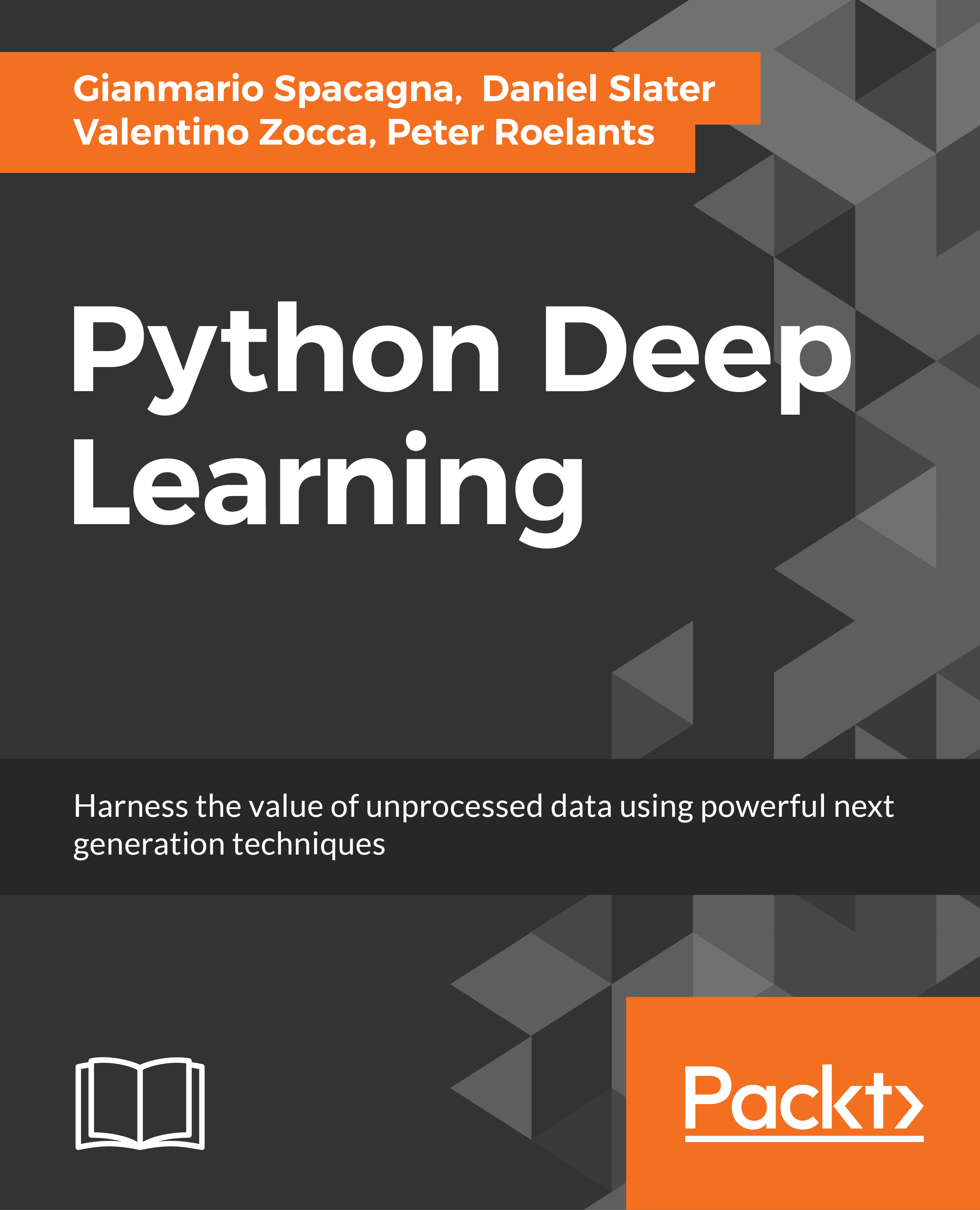
Python Deep Learning
$60.99
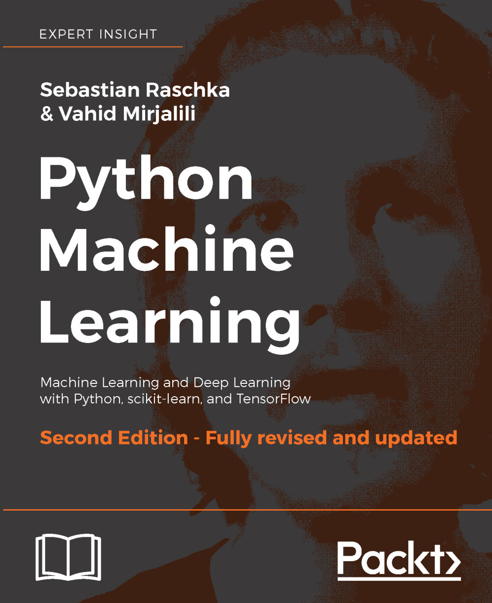
Python Machine Learning, Second Edition
$43.99
Python Deep Learning Cookbook
$48.99
Total $ 153.97 Stars icon
Banner background image

Table of Contents

14 Chapters
Programming Environments, GPU Computing, Cloud Solutions, and Deep Learning Frameworks Chevron down icon Chevron up icon
Feed-Forward Neural Networks Chevron down icon Chevron up icon
Convolutional Neural Networks Chevron down icon Chevron up icon
Recurrent Neural Networks Chevron down icon Chevron up icon
Reinforcement Learning Chevron down icon Chevron up icon
Generative Adversarial Networks Chevron down icon Chevron up icon
Computer Vision Chevron down icon Chevron up icon
Natural Language Processing Chevron down icon Chevron up icon
Speech Recognition and Video Analysis Chevron down icon Chevron up icon
Time Series and Structured Data Chevron down icon Chevron up icon
Game Playing Agents and Robotics Chevron down icon Chevron up icon
Hyperparameter Selection, Tuning, and Neural Network Learning Chevron down icon Chevron up icon
Network Internals Chevron down icon Chevron up icon
Pretrained Models Chevron down icon Chevron up icon

Customer reviews

Rating distribution
Full star icon Full star icon Full star icon Half star icon Empty star icon 3.7
(3 Ratings)
5 star 66.7%
4 star 0%
3 star 0%
2 star 0%
1 star 33.3%
Gert Dec 30, 2017
Full star icon Full star icon Full star icon Full star icon Full star icon 5
positive points:• The book builds on simple recipes toward more complex recipes.• Great book if you want to learn by example!• A lot of useful code is included in the book that you can reuse for different projects.• What I like is that the author focusses on experimentation and doesn’t assume one method is better over another.negative points:• Sometimes a bit more explanation why some of the choices have been made would be good.• It would be better if the images are in colour (especially some charts).
Amazon Verified review Amazon
newby19 Nov 19, 2017
Full star icon Full star icon Full star icon Full star icon Full star icon 5
I think this book is a great way to get started using deep learning in a hands-on way. Especially for someone who's relatively new to deep learning and wants to experiment and work on different projects.Each recipe in the book is broken down to the different steps to take. Each step is described shortly and to the point. I used the recipes from the Computer Vision chapter right away to create my own image classification project.
Amazon Verified review Amazon
Some Python Guy Dec 19, 2017
Full star icon Empty star icon Empty star icon Empty star icon Empty star icon 1
Found the code files on git but for example the wav/video files from chapter 9 are missing. Likely other source data files are missing. Please provide all relevant input files to run the samples.
Amazon Verified review Amazon
Get free access to Packt library with over 7500+ books and video courses for 7 days!
Start Free Trial

FAQs

What is the delivery time and cost of print book? Chevron down icon Chevron up icon

Shipping Details

USA:

'

Economy: Delivery to most addresses in the US within 10-15 business days

Premium: Trackable Delivery to most addresses in the US within 3-8 business days

UK:

Economy: Delivery to most addresses in the U.K. within 7-9 business days.
Shipments are not trackable

Premium: Trackable delivery to most addresses in the U.K. within 3-4 business days!
Add one extra business day for deliveries to Northern Ireland and Scottish Highlands and islands

EU:

Premium: Trackable delivery to most EU destinations within 4-9 business days.

Australia:

Economy: Can deliver to P. O. Boxes and private residences.
Trackable service with delivery to addresses in Australia only.
Delivery time ranges from 7-9 business days for VIC and 8-10 business days for Interstate metro
Delivery time is up to 15 business days for remote areas of WA, NT & QLD.

Premium: Delivery to addresses in Australia only
Trackable delivery to most P. O. Boxes and private residences in Australia within 4-5 days based on the distance to a destination following dispatch.

India:

Premium: Delivery to most Indian addresses within 5-6 business days

Rest of the World:

Premium: Countries in the American continent: Trackable delivery to most countries within 4-7 business days

Asia:

Premium: Delivery to most Asian addresses within 5-9 business days

Disclaimer:
All orders received before 5 PM U.K time would start printing from the next business day. So the estimated delivery times start from the next day as well. Orders received after 5 PM U.K time (in our internal systems) on a business day or anytime on the weekend will begin printing the second to next business day. For example, an order placed at 11 AM today will begin printing tomorrow, whereas an order placed at 9 PM tonight will begin printing the day after tomorrow.


Unfortunately, due to several restrictions, we are unable to ship to the following countries:

  1. Afghanistan
  2. American Samoa
  3. Belarus
  4. Brunei Darussalam
  5. Central African Republic
  6. The Democratic Republic of Congo
  7. Eritrea
  8. Guinea-bissau
  9. Iran
  10. Lebanon
  11. Libiya Arab Jamahriya
  12. Somalia
  13. Sudan
  14. Russian Federation
  15. Syrian Arab Republic
  16. Ukraine
  17. Venezuela
What is custom duty/charge? Chevron down icon Chevron up icon

Customs duty are charges levied on goods when they cross international borders. It is a tax that is imposed on imported goods. These duties are charged by special authorities and bodies created by local governments and are meant to protect local industries, economies, and businesses.

Do I have to pay customs charges for the print book order? Chevron down icon Chevron up icon

The orders shipped to the countries that are listed under EU27 will not bear custom charges. They are paid by Packt as part of the order.

List of EU27 countries: www.gov.uk/eu-eea:

A custom duty or localized taxes may be applicable on the shipment and would be charged by the recipient country outside of the EU27 which should be paid by the customer and these duties are not included in the shipping charges been charged on the order.

How do I know my custom duty charges? Chevron down icon Chevron up icon

The amount of duty payable varies greatly depending on the imported goods, the country of origin and several other factors like the total invoice amount or dimensions like weight, and other such criteria applicable in your country.

For example:

  • If you live in Mexico, and the declared value of your ordered items is over $ 50, for you to receive a package, you will have to pay additional import tax of 19% which will be $ 9.50 to the courier service.
  • Whereas if you live in Turkey, and the declared value of your ordered items is over € 22, for you to receive a package, you will have to pay additional import tax of 18% which will be € 3.96 to the courier service.
How can I cancel my order? Chevron down icon Chevron up icon

Cancellation Policy for Published Printed Books:

You can cancel any order within 1 hour of placing the order. Simply contact customercare@packt.com with your order details or payment transaction id. If your order has already started the shipment process, we will do our best to stop it. However, if it is already on the way to you then when you receive it, you can contact us at customercare@packt.com using the returns and refund process.

Please understand that Packt Publishing cannot provide refunds or cancel any order except for the cases described in our Return Policy (i.e. Packt Publishing agrees to replace your printed book because it arrives damaged or material defect in book), Packt Publishing will not accept returns.

What is your returns and refunds policy? Chevron down icon Chevron up icon

Return Policy:

We want you to be happy with your purchase from Packtpub.com. We will not hassle you with returning print books to us. If the print book you receive from us is incorrect, damaged, doesn't work or is unacceptably late, please contact Customer Relations Team on customercare@packt.com with the order number and issue details as explained below:

  1. If you ordered (eBook, Video or Print Book) incorrectly or accidentally, please contact Customer Relations Team on customercare@packt.com within one hour of placing the order and we will replace/refund you the item cost.
  2. Sadly, if your eBook or Video file is faulty or a fault occurs during the eBook or Video being made available to you, i.e. during download then you should contact Customer Relations Team within 14 days of purchase on customercare@packt.com who will be able to resolve this issue for you.
  3. You will have a choice of replacement or refund of the problem items.(damaged, defective or incorrect)
  4. Once Customer Care Team confirms that you will be refunded, you should receive the refund within 10 to 12 working days.
  5. If you are only requesting a refund of one book from a multiple order, then we will refund you the appropriate single item.
  6. Where the items were shipped under a free shipping offer, there will be no shipping costs to refund.

On the off chance your printed book arrives damaged, with book material defect, contact our Customer Relation Team on customercare@packt.com within 14 days of receipt of the book with appropriate evidence of damage and we will work with you to secure a replacement copy, if necessary. Please note that each printed book you order from us is individually made by Packt's professional book-printing partner which is on a print-on-demand basis.

What tax is charged? Chevron down icon Chevron up icon

Currently, no tax is charged on the purchase of any print book (subject to change based on the laws and regulations). A localized VAT fee is charged only to our European and UK customers on eBooks, Video and subscriptions that they buy. GST is charged to Indian customers for eBooks and video purchases.

What payment methods can I use? Chevron down icon Chevron up icon

You can pay with the following card types:

  1. Visa Debit
  2. Visa Credit
  3. MasterCard
  4. PayPal
What is the delivery time and cost of print books? Chevron down icon Chevron up icon

Shipping Details

USA:

'

Economy: Delivery to most addresses in the US within 10-15 business days

Premium: Trackable Delivery to most addresses in the US within 3-8 business days

UK:

Economy: Delivery to most addresses in the U.K. within 7-9 business days.
Shipments are not trackable

Premium: Trackable delivery to most addresses in the U.K. within 3-4 business days!
Add one extra business day for deliveries to Northern Ireland and Scottish Highlands and islands

EU:

Premium: Trackable delivery to most EU destinations within 4-9 business days.

Australia:

Economy: Can deliver to P. O. Boxes and private residences.
Trackable service with delivery to addresses in Australia only.
Delivery time ranges from 7-9 business days for VIC and 8-10 business days for Interstate metro
Delivery time is up to 15 business days for remote areas of WA, NT & QLD.

Premium: Delivery to addresses in Australia only
Trackable delivery to most P. O. Boxes and private residences in Australia within 4-5 days based on the distance to a destination following dispatch.

India:

Premium: Delivery to most Indian addresses within 5-6 business days

Rest of the World:

Premium: Countries in the American continent: Trackable delivery to most countries within 4-7 business days

Asia:

Premium: Delivery to most Asian addresses within 5-9 business days

Disclaimer:
All orders received before 5 PM U.K time would start printing from the next business day. So the estimated delivery times start from the next day as well. Orders received after 5 PM U.K time (in our internal systems) on a business day or anytime on the weekend will begin printing the second to next business day. For example, an order placed at 11 AM today will begin printing tomorrow, whereas an order placed at 9 PM tonight will begin printing the day after tomorrow.


Unfortunately, due to several restrictions, we are unable to ship to the following countries:

  1. Afghanistan
  2. American Samoa
  3. Belarus
  4. Brunei Darussalam
  5. Central African Republic
  6. The Democratic Republic of Congo
  7. Eritrea
  8. Guinea-bissau
  9. Iran
  10. Lebanon
  11. Libiya Arab Jamahriya
  12. Somalia
  13. Sudan
  14. Russian Federation
  15. Syrian Arab Republic
  16. Ukraine
  17. Venezuela