Solution 1 – logic tensor networks
In our first Python NSAI example, we will implement a system based on the Logic Tensor Network (LTN) framework.
In short, LTNs are a sub-class of neural networks that leverage logical propositions (i.e., symbolic logic). LTNs use logical propositions to represent the knowledge base as formulas and deep learning to learn the different weights of these formulas. These logical propositions act as soft constraints on the neural network’s inference. If the neural network’s output violates the logical propositions, then it is penalized. As a result, an LTN during training has two main objectives: 1) satisfy the logical propositions, and 2) improve its predictive performance on the target objective. As such, the logical propositions as model constraints act as a way to directly integrate prior domain knowledge into the neural network.
For the more interested reader, you can read the full LTN paper at https://arxiv.org/pdf/1606.04422.pdf.
The first objective is, therefore, to correctly represent our dataset (i.e., the knowledge base) as logical formulas. In LTNs, we typically represent these logical formulas as axioms.
Defining an axiom
An axiom is a logical statement that is the general (and accepted) truth. Axioms are typically taken to be true without any proof and should be simple enough to be self-evident. Axioms can comprise connectives, predicates, terms, or propositions (or a mix).
For example, “if you add zero to any number, the result is always that same number” is an axiom.
We use these axioms to build a vector space of knowledge (i.e., we extend the first-order logical statements by representing them as multi-dimension vectors – from logical statements to tensors). We refer to this concept as grounding. The motivation behind the vector space representation is to enable relationship mapping and reasoning between the different logical statements, as opposed to True or False values supported by the axioms. This process is called real logic and is the core concept of LTNs.
In this chapter, we do not define or discuss the formal mathematical definitions of LTNs. Additionally, we will use the excellent Python library LTNtorch (https://github.com/tommasocarraro/LTNtorch). LTNtorch is an LTN implementation based on the deep learning package PyTorch (https://github.com/pytorch/pytorch). LTNtorch also comprehensively explains the mathematical foundations around the LTN algorithm.
Loading the dataset
First things first, let us install this package in our environment. In Colab, we can use the ! operator to directly execute terminal commands from within the Python cell, as follows:
!pip install LTNtorch
Next, we want to import the required libraries. In this example, we need the following packages:
import torch
import ltn
import numpy as np
from sklearn.metrics import accuracy_score
At this point, we have already loaded our dataset. The remaining step is to split the dataset into features and labels and then split them into training and testing sets. For now, let us split the features:
features = df.drop('Class_att', axis=1).values
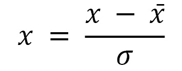
We will also standardize our features to have a zero mean and unit variance (i.e., a variance equal to 1). This step has several benefits. Mainly to remove scale influence (for example, the disparity between a feature measuring a person’s age and another calculating their salary) and to help the NN converge faster (i.e., faster training). We use the following equation to perform this step:

Where  denotes the observation,
  denotes the sample mean of
  , and
, and  denotes the sample standard deviation of
  :
:
# standardize our features
features = (features - features.mean()) / features.std()
Modifying the dataset
We will now split the labels and transform both features and labels into tensors directly using the PyTorch library. Again, we simply drop our label column (i.e., style) for our feature set. This time, we do not want the operation to be done in place. Instead, we want to return a new DataFrame. If we did this operation in place, then we would be overwriting our original DataFrame and therefore losing our label column. We call the .values property to return a NumPy representation of the DataFrame.
We load both features and labels as PyTorch tensors by calling the torch.tensor() function. We use the .to() function to specify the data type of our tensors:
# convert our features and labels to tensors
features = torch.tensor(features).to(dtype=torch.float32)
labels = torch.tensor(df['style'].values).to(dtype=torch.float32)
Creating train and test datasets
We’ll now create our training and testing sets. We’ll use PyTorch’s DataLoader functionality to do so. The DataLoader allows us to pass batches of the dataset to our NN. We’ll define a standard PyTorch DataLoader (read more at https://pytorch.org/docs/stable/data.html#torch.utils.data.DataLoader).
We create the class structure using the following:
class DataLoader(object):
The above DataLoader class must define three main functions:
__init__: The constructor for the class. It describes the different properties that every instance of that class can have. The main properties we are after are the data (i.e., our features), the labels, the batch size, and whether we want to shuffle the samples. We can implement it as follows:
def __init__(self, data, labels, batch_size=1, shuffle=True):
    self.data = data
    self.labels = labels
    self.batch_size = batch_size
    self.shuffle = shuffle
__len__: Logic to execute whenever we call the len() function on any instance of this class. This definition helps us determine the number of batches based on a specified batch size.
We divide the total number of samples (obtained using .shape[0]) by the specified batch size. We take the result’s ceil (i.e., round up to the nearest integer value) as our total number of batches. This function looks like this:
def __len__(self):
    return int(np.ceil(self.data.shape[0] / self.batch_size))
__iter__: Describes the logic to run when we iterate over any instance of this class. This function is also used throughout the batching process.
This function needs to be an iterator. Based on our batch size, it should yield a series of batches from our features and labels. When creating our batches, keeping the number of samples from the different labels as balanced as possible is vital. For example, we only have two labels in our binary classification task. Therefore, we first separate and shuffle our samples based on their label:
def __iter__(self):
    n = self.data.shape[0]
    idx_pos = np.where(self.labels == 1)[0]
    idx_neg = np.where(self.labels == 0)[0]
    np.random.shuffle(idx_pos)
    np.random.shuffle(idx_neg)
Then, we choose an equal (or fewer if there are not enough samples) subset of samples from both labels randomly per batch:
    for start_idx in range(0, n, self.batch_size):
        end_idx = min(start_idx + self.batch_size, n)
        # Get one positive and one negative sample for each batch
        pos_batch_size = min(self.batch_size // 2, len(idx_pos))
        neg_batch_size = self.batch_size - pos_batch_size
        pos_idx = idx_pos[:pos_batch_size]
        neg_idx = np.random.choice(idx_neg, size=neg_batch_size,                                   replace=False)
Finally, we concatenate the results, reshuffle them, and produce the features and labels for that batch:
        idx = np.concatenate([pos_idx, neg_idx])
        np.random.shuffle(idx)
        data = self.data[idx]
        labels = self.labels[idx]
        yield data, labels
We take the first 91 samples as part of our training set and the remaining for testing. There is no specific reasoning behind the decision to take the first 91 samples for training. One can experiment with different percentage allocations between the training and testing sets. We restrict the training set to such a small amount to highlight the power of NSAI when it comes to small data. Of course, in the real world, it would be ideal to use all the data in our possession:
# create training and testing dataloader, batch_size = 64
train_loader = DataLoader(features[:91], labels[:91], 64, True)
test_loader = DataLoader(features[91:], labels[91:], 64, False)
Defining our knowledge base and NN architecture
The next step is to extract the knowledge base (axioms) and create our NN. We define our predicate, the connectives, and the quantifiers.
Giving context to predicates, connectives, and quantifiers
Predicate: In LTNs, an algorithm maps a high-dimensional vector space to a specific label set. Our binary classification task requires the predicate to map to either 0 or 1.
Connective: A logical connective such as a conjunction (AND), disjunction (OR), negation (NOT), or implication (IMPLIES).
Quantifier: Describes how many (i.e., the quantity) samples satisfy the predicate. The two main quantifiers are Universal (indicates the for all amount, represented by the symbol ∀) and Existential (indicates the exists quantity, represented by the symbol ∃).
For our example, we define our predicate as a simple feed-forward NN using PyTorch (refer to Figure 8.1). We create a network with an input layer translating the dataset’s 11 features to 64 neurons, a hidden layer with 64 neurons, and an output layer converging to a single neuron.

Figure 8.1: The architecture used for our simple feed-forward NN
The network hyperparameter tuning procedure includes choosing the number of neurons per layer, which is often a trial-and-error process. We use the Rectified Linear Unit (ReLU) function to activate the input and hidden layers and the sigmoid function to limit the output of the output layer to the [0, 1] range. This is a standard architecture for most binary classification tasks:
# we define predicate A
class ModelA(torch.nn.Module):
    def __init__(self):
        super(ModelA, self).__init__()
        self.sigmoid = torch.nn.Sigmoid()
        self.layer1 = torch.nn.Linear(11, 64)
        self.layer2 = torch.nn.Linear(64, 64)
        self.layer3 = torch.nn.Linear(64, 1)
        self.relu = torch.nn.ReLU()
        self.dropout = torch.nn.Dropout(p=0.1)
    def forward(self, x):
        x = self.relu(self.layer1(x))
        x = self.relu(self.layer2(x))
        x = self.dropout(x)
        return self.sigmoid(self.layer3(x))
We keep the NN implementation simple for the sake of explanation. Moreover, our dataset is tiny, making it easy to overfit (i.e., the model fit is too close to the training data – essentially it would perform very well during training but significantly worse on unseen data) with unnecessarily complex networks. The predicate function (i.e., our deep learning component) would likely become increasingly difficult with more complex data structures and knowledge bases. One might also experiment with different NN architectures, for example, a convolutional NN (CNN).
Defining our predicate, connectives, and quantifiers
Next, we define our connectives and quantifiers. Implementing these is easy in LTNtorch. We define a NOT connective and a FOR ALL quantifier. These are the recommended settings by LTNtorch for binary classification. It is wise to dive deeper into the package’s various options for more complex use cases to determine the correct configuration for your dataset:
# create our predicate (i.e., our NN)
A = ltn.Predicate(ModelA())
# create the NOT standard connective
Not = ltn.Connective(ltn.fuzzy_ops.NotStandard())
# create the FOR ALL quantifier
Forall = ltn.Quantifier(ltn.fuzzy_ops.AggregPMeanError(p=2),
                        quantifier="f")
We define the FOR ALL quantifier by specifying the quantifier parameter as f.
Here, the connective module contributes to the knowledge-base extraction by amalgamating sub-formulas with different features. The quantifier module determines the formula dimensions for tensor aggregation.
We are almost there!
Setting up evaluation parameters
Before we can train our LTN, we need a way to evaluate our system. We need to evaluate two aspects of the architecture.
The knowledge-base satisfaction level (the SAT level)
This metric answers the question of how good the LTN is at learning. We will use this throughout the training process as part of our loss function (we want to maximize this metric).
We can iterate over our data samples and split them based on their label. Then, per the label, we can compute the SAT level using the SatAgg function provided by LTNtorch by comparing the true samples with the predicted results from our NN:
def compute_sat_level(loader):
    mean_sat = 0
    for data, labels in loader:
        # get our positive samples
        x_A = ltn.Variable("x_A",data[torch.nonzero(labels)])
        # get our negative samples
        x_not_A = ltn.Variable("x_not_A", data[torch.nonzero(                                          torch.logical_not(labels))])
Finally, we take the mean of the two SAT levels and repeat until we iterate over all samples:
        # get the mean SAT of both sample types
        mean_sat += SatAgg(Forall(x_A, A(x_A)),
                           Forall(x_not_A, Not(A(x_not_A)))
        )
    # get the mean SAT over all samples
    mean_sat /= len(loader)
    return mean_sat
The classification performance
This metric gives the overall performance of the model.
For our simple example, we will use the accuracy score implemented by sklearn (read more at https://scikit-learn.org/stable/modules/model_evaluation.html#accuracy-score). Depending on the use case, you might want to monitor one or more different metrics.
We iterate over all samples and measure the mean accuracy score by comparing the true labels and their respective predicted labels:
def compute_accuracy(loader):
    mean_accuracy = 0.0
    # iterate over our data samples
    for data, labels in loader:
        # get the predictions for the given samples
        predictions = A.model(data).detach().numpy()
        # convert to a binary classification (i.e., 0 or 1)
        predictions = np.where(predictions > 0.5, 1., 0.).flatten()
        # compute the accuracy_score
        mean_accuracy += accuracy_score(labels, predictions)
    # get the mean accuracy
    return mean_accuracy / len(loader)
We must also initialize a SatAgg object from the LTNtorch package to aggregate the SAT levels. At this step, we can also define the optimizer for our NN. We will use the standard Adam optimizer with a learning rate of 0.001. The Adam optimizer is an algorithm that optimizes the stochastic gradient descent process. In short, it is used to adjust the learning rate of NN throughout the training process:
SatAgg = ltn.fuzzy_ops.SatAgg()
optimizer = torch.optim.Adam(A.parameters(), lr=0.001)
Now, we are ready to train our LTN.
Training the LTN model
The training process is split as follows. First, we will start batching the data we created earlier for a certain number of epochs (i.e., iterations):
EPOCHS: int = 100
for epoch in range(EPOCHS):
    # reset the training loss for every epoch
    train_loss = 0.0
    # start batching the data
    for batch_idx, (data, labels) in enumerate(train_loader):
Per batch, we split the positive and negative samples into their respective variables and measure their individual SAT level using the created FOR ALL quantifier. We also need to call the zero_grad() function to set the gradients to zero before starting the backpropagation of the training process. This step is a standard process in the PyTorch library (to know more, you can have a look at this well-formulated Stack Overflow answer https://stackoverflow.com/a/48009142/4587043):
        optimizer.zero_grad()
        # we ground the variables with current batch data
        x_A = ltn.Variable("x_A", data[torch.nonzero(labels)])
        # positive examples
        x_not_A = ltn.Variable("x_not_A", data[torch.nonzero(                               torch.logical_not(labels))])
        # negative examples
        # compute SAT level
        sat_agg = SatAgg(Forall(x_A, A(x_A)),
                         Forall(x_not_A, Not(A(x_not_A)))
        )
Then, we calculate our loss value (by subtracting the computed SAT level from 1) and train the NN using back-propagation. This step helps us monitor the error margin in our SAT predictions. The smaller the loss value, the better our NN is performing. As such, we want to optimize learning by minimizing the loss value:
        # compute loss and perform back-propagation
        loss = 1. - sat_agg
        loss.backward()
        optimizer.step()
        train_loss += loss.item()
After iterating over all batches, we monitor the current training loss and print to console the current results on every 20th epoch:
    # monitor the training loss
    train_loss = train_loss / len(train_loader)
    # we print metrics every 20 epochs of training
    if epoch % 20 == 0:
        print(" epoch %d | loss %.4f | Train Sat %.3f | Test Sat %.3f | Train Acc %.3f | Test Acc %.3f"
            %(epoch, train_loss,
                compute_sat_level(train_loader),
                compute_sat_level(test_loader),
                compute_accuracy(train_loader),
                compute_accuracy(test_loader)))
Analyzing the results
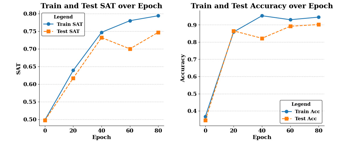
Monitoring the training process, the SAT and accuracy scores improve with every epoch.

Figure 8.2: Train and test SAT (left) and accuracy (right) scores over the epochs
The preceding plots highlight an exciting benefit of LTNs, which we have already discussed in the previous chapters. The NSAI architecture generalizes quickly and arguably better (i.e., the model’s performance on the unseen data is improved), resulting in a rapid training process. After 80 epochs, we reached an accuracy score of around 90% on the test set. However, after just 20 epochs, we got an accuracy figure of approximately 87% (starting at just under 35% at epoch 0). Considering that our training dataset consists of only 91 samples, this highlights the power of NSAI to achieve high performance with small data. The influence of LTNs in obtaining such predictive performance is also worth noting, with the only training objective being knowledge satisfaction. Including prior knowledge in training therefore improves the model’s fit – especially in unseen cases. If we were to run the same training process using a training set of 5,000 samples (around 75% of the entire dataset), our results wouldn’t vary too much. After 80 epochs, we obtain a testing accuracy score of around 92.3% (at the 20th epoch, we were already at 91.7%). Although increasing the number of training data samples did improve our model’s performance, we must appreciate the performance obtained with training on just 91 random samples. Out in the real world, this difference in training sizes might translate to millions of dollars saved from overheads to see the entire training process through.
Granted, this task is a straightforward one and others have easily obtained 99% accuracy. However, if we compare these results against other documented ones, we can quickly start to appreciate the NSAI benefit of needing significantly smaller data to learn and less complex NN architectures. A similar experiment to ours based on NNs (https://www.kaggle.com/code/hhp07022000/wine-quality-prediction-and-type-classification) reached 99% accuracy after training for 700 epochs. It is also worth noting that the NN used in this experiment had double the size (with 128 neurons in the hidden layer compared to our 64). On larger-scale projects, these implications will have a significant value.
Another benefit of LTNs (and subsequently, NSAI) is their high transparency. We have stated multiple times that NSAI systems are explainable by default. The LTN training process involves translating first-order logic to tensor embeddings. We start off with logical relationships between variables and predicates. Then, we use quantifiers over the variables and predicates (returning either True or False) and transform them into multi-dimensional vectors (using tensor operations). As such, the resulting tensors embed the logical relationships. We can trace the entire process for every prediction by examining the tensor operations and logical connections.
Of course, out in the real world, the process would not be complete here. Instead, it typically involves a lot of back-and-forth experimenting with different hyperparameters to minimize over-fitting and improve model robustness.


