Search icon CANCEL
Subscription
0
Cart icon
Your Cart (0 item)
Close icon
You have no products in your basket yet
Save more on your purchases! discount-offer-chevron-icon
Savings automatically calculated. No voucher code required.
Arrow left icon
Explore Products
Best Sellers
New Releases
Books
Videos
Audiobooks
Learning Hub
Newsletter Hub
Free Learning
Arrow right icon
timer SALE ENDS IN
0 Days
:
00 Hours
:
00 Minutes
:
00 Seconds
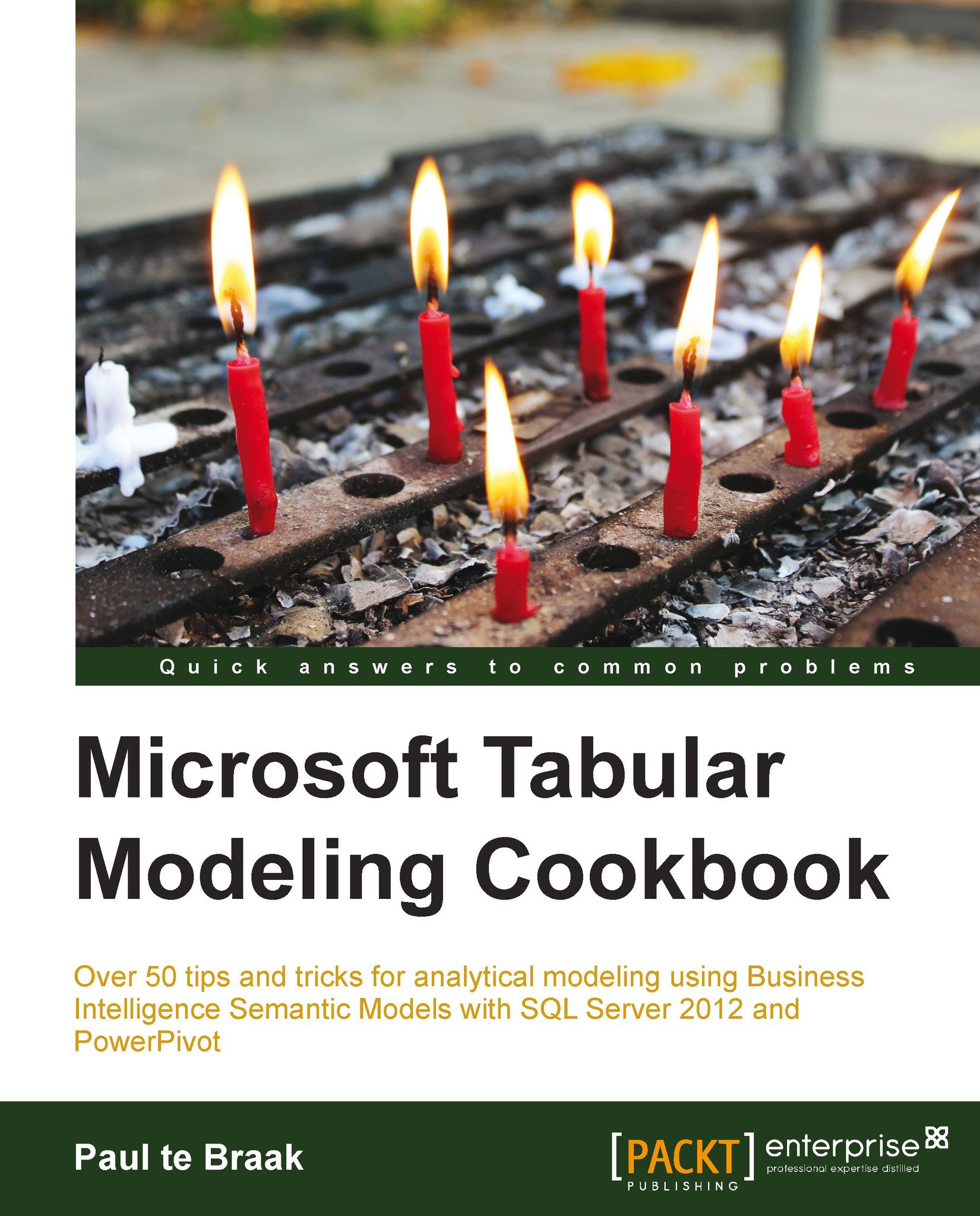
Microsoft Tabular Modeling Cookbook

Microsoft Tabular Modeling Cookbook: No prior knowledgeof tabular modeling is needed to benefit from this brilliant cookbook. This is the total guide to developing and managing analytical models using the Business Intelligence Semantic Models technology.

Arrow left icon
Profile Icon te Braak
Arrow right icon
Mex$179.99 Mex$1000.99
Full star icon Full star icon Full star icon Full star icon Half star icon 4.7 (7 Ratings)
eBook Dec 2013 320 pages 1st Edition
eBook
Mex$179.99 Mex$1000.99
Paperback
Mex$1251.99
Subscription
Free Trial
Arrow left icon
Profile Icon te Braak
Arrow right icon
Mex$179.99 Mex$1000.99
Full star icon Full star icon Full star icon Full star icon Half star icon 4.7 (7 Ratings)
eBook Dec 2013 320 pages 1st Edition
eBook
Mex$179.99 Mex$1000.99
Paperback
Mex$1251.99
Subscription
Free Trial
eBook
Mex$179.99 Mex$1000.99
Paperback
Mex$1251.99
Subscription
Free Trial

What do you get with eBook?

Product feature icon Instant access to your Digital eBook purchase
Product feature icon Download this book in EPUB and PDF formats
Product feature icon Access this title in our online reader with advanced features
Product feature icon DRM FREE - Read whenever, wherever and however you want
OR
Modal Close icon
Payment Processing...
tick Completed

Billing Address

Table of content icon View table of contents Preview book icon Preview Book

Microsoft Tabular Modeling Cookbook

Chapter 1. Getting Started with Excel

In this chapter, we will cover:

  • Creating the model
  • Managing the appearance of tables and fields
  • Using tabular relationships to filter data
  • Adding fields to tables
  • Linking fields between tables
  • Creating model calculations

Introduction

This chapter is designed as an introduction to tabular modeling by using PowerPivot. It shows the process by which a user imports data into PowerPivot for Excel, creates relationships between the datasets, and then reports on it.

The data used in this chapter is based on the orders of the fictitious bicycle company (named Adventure Works). Our data includes six datasets and they are:

  • Product list: This shows some generic information about the products being sold (for example, the name, color, and size of the product). Each product is identified by a product_id value.
  • Product subcategories list: This shows a subcategory that a product belongs to. The list shows the product_id value and the associated subcategory (by ID and Name).
  • Product categories list: This shows the product category that a product belongs to. The list shows the product_id value and the associated category (by ID and Name).
  • Orders list: This shows what orders have been placed by customers. The list includes an entry for each product that has been ordered. This data simulates a detailed extract from an operational source system.
  • Customer list: This gives us information about the customer (for example, their names, countries, and states) by customer number.
  • Dates list: This simply lists consecutive days defining information such as the month name, year, and half-year period of the date.

The tabular modeling lifecycle revolves around three primary steps. These are:

  • Getting the data into the model
  • Defining the relationships among tables
  • Defining calculations based on business logic

This chapter examines these steps and allows the reader to become familiar with the tabular (PowerPivot) design environment.

Creating the model

An Excel workbook can only contain one tabular model and that one model contains tables of data (which may or may not be related). The first step to create a model is to import data into it. There are many techniques to do this—some techniques have advantages over others but for now, let's only consider the fact that we want to load data that exists in an Excel worksheet into the model.

Tip

The installation instructions for PowerPivot in Excel 2010 are covered in the Appendix, Installing PowerPivot and Sample Databases, of this book.

Getting ready

Open the Excel workbook named SalesBook which is available from the Packt Publishing website to examine the worksheets within the book. Each sheet contains a dataset for Products, Subcategories, Categories, Customers, Dates, and Sales.

How to do it…

This recipe looks at importing data into the PowerPivot model through linked tables. These are very convenient to use when the data is stored in Excel. Additionally, once the data has been imported into PowerPivot, it retains a connection to the Excel table. This means that, when the data is changed in Excel, it can also be changed in the PowerPivot model.

  1. Let's start by importing the product list. Select the Product List sheet and select cell A1.
  2. Then, on the PowerPivot tab, click on the Create Linked Table button.

    Tip

    Excel will automatically highlight the data range.

    How to do it…
  3. A small window will open confirming the data range with a checkbox for table headers. Select the checkbox and press OK.
  4. The PowerPivot window will open and the data from the Product List sheet will be imported. Note that the table appears as a tab which is similar to Excel and is called Table1. Also, note that the PowerPivot window is a separate window than the Excel workbook, so that we can return to Excel.
    How to do it…
  5. Repeat this process for all the remaining datasets except Customers.

How it works…

When a linked table is created in PowerPivot, Excel creates a named range in the Excel workbook. This is then linked to the PowerPivot model (note that there is a small chain symbol before each of the tables). Also, note that the tables in Excel are formatted with alternate blue coloring. The named ranges can be viewed in Excel by clicking on the Name Manager button on the Formulas tab.

How it works…

There's more…

A table (table range) is actually an Excel feature that PowerPivot utilizes. A table can be defined in Excel, given a meaningful name and then imported into PowerPivot, so that the name of the table in PowerPivot is the same as the named range in Excel.

Ensure that the Customers sheet is selected in Excel and also any cell in the Customers data is selected. In the Home tab, click on the Format as Table button, and choose a table style; the style chosen in the following screenshot is a relevant one:

There's more…

Note that the data is now formatted with alternating colors (based on the selected style). Return to the Name Manager window and double-click the table that relates to the Customers worksheet. A new window will open allowing you to edit the name, replace the name Table6 with Customers, and click on OK. The Table6 name is replaced by Customers in the Name Manager window.

There's more…

Now, create a linked table in the same manner as we did before and note that the name of the table imported into PowerPivot is Customers.

Tip

If you want to select an entire table in Excel, simply choose the table name from the Name Box drop-down list in the formula bar in the upper-left corner. This is shown in the following screenshot:

There's more…

Managing the appearance of tables and fields

A PowerPivot workbook contains two products that allow the user to analyze data. Firstly, there is the xVelocity in-memory analytics engine (the tabular model) which is a columnar database embedded in the workbook. Secondly, there is a client tool that allows the model to be queried, it also displays the results to the user in the form of a pivot table or pivot chart. In Excel 2010, the client tool was restricted to pivot table functionality (for example, a pivot table or pivot chart). In Excel 2013, the tools set has been extended to include Power View. The important distinction here is that the client tool is used to present the model to the user. This recipe shows how to control the way the model is presented to the user.

Getting ready

This recipe uses the model that has already been created in the prior recipe Creating the model. If this model has not been created, follow the recipe to ensure that the model has been loaded with data.

How to do it…

Start from an existing model within PowerPivot.

  1. Ensure that you are in the PowerPivot window (not Excel), then click on the PivotTable button in the Home Tab.
    How to do it…
  2. PowerPivot will switch back to the Excel window and a dialog will prompt for the location of the new pivot table. Select New Worksheet and click on OK.
    How to do it…
  3. Excel will now show PowerPivot Field List and a pivot table work area. These are identified by the arrows in the following screenshot. Note that PowerPivot Field List shows tables from the model as nodes, with the fields from the model as children.
    How to do it…
  4. Return to the PowerPivot application window and double-click on the Table1 tab. The name Table1 will be in a blue background and rename it to Products. Repeat this exercise for the other tables (Subcategory, Category, Dates, and Sales). The table names in your PowerPivot window will now look like the following screenshot:
    How to do it…
  5. Return to Excel and notice that PowerPivot Field List has detected a change in the model and prompts the user to refresh. Click on the Refresh button and note that the changes in the names of the tables are now reflected in the PowerPivot Field List panel.

    Before

    After

    How to do it…
    How to do it…
  6. Return to the PowerPivot application window and select the Products table. Double-click on the product_id field and enter Product ID as the new name. The field will have a blue background when its name can be changed.
    How to do it…
  7. Return to the PowerPivot window and update the remaining columns to the following names:

    Table

    Column

    New name

    Products

    product_id

    Product ID

    Products

    product_name

    Product Name

    Products

    colour

    Colour

    Products

    size_range

    Size Range

    Products

    size

    Size

    Subcategory

    subcategory_name

    Subcategory

    Category

    category_name

    Category

    Dates

    date

    Day

    Dates

    year

    Year

    Dates

    month_name

    Month

    Dates

    half_name

    Half

    Sales

    order_number

    SO Number

    Customers

    customer_id

    Customer ID

    Customers

    customer_name

    Customer Name

    Customers

    country_code

    Country Code

    Customers

    state_code

    State Code

  8. Return to Excel and refresh PowerPivot Field List. The column names will now display as those that were entered.

    Tip

    You can also rename fields by right-clicking on the field and selecting Rename Column from the pop-up in PowerPivot. Alternatively, you can double-click on the field name (so that it changes the color of the field) and rename it.

  9. Return to the PowerPivot window and select the Sales table. Right-click anywhere on the order_number_line field and select Hide from Client Tools in the pop-up window. Select all the fields product_id, order_date, and customer_id by clicking-and-dragging the mouse across the three fields and hide these fields too.

    Tip

    PowerPivot mimics Excel in the way that you can select multiple fields by dragging your mouse across several columns (with the left button continually pressed). You can also select the first column, hold the Shift key, and select the final column.

    Unlike Excel, multiple columns cannot be selected by using the Ctrl key and selecting multiple fields.

  10. Return to the PowerPivot window, refresh PowerPivot Field List, and expand the Sales table. Note that these fields no longer appear in the field list.
  11. Add the Day field to the pivot by expanding the Dates table and selecting the checkbox next to the Day field. The column will be automatically added to the rows area of the pivot and will be displayed, as shown in the following screenshot:
    How to do it…

    Tip

    You can achieve the same result by dragging the Day field and dropping it in the Row Labels area of the pivot.

  12. Return to the PowerPivot window and select the Day column. From the format list, select More Dates Formats…, and then select the dd-MMM-yy format from the list of available formats. The value presented will show a formatted sample of the data. Choose the item that shows 14-Mar-01.
    How to do it…
  13. Return to Excel and refresh the pivot table. Note that the PowerPivot Field List panel may not indicate the change to the model. However, when the pivot table is refreshed, the data displays the new format.
    How to do it…
  14. In the Sales table, format the columns unit_price, unit_cost, tax, and total_price as a whole numeric number by selecting the columns and choosing Currency from the Format drop-down list.

How it works…

The semantic model defines the metadata structure of the model and includes information such as table names, column names, and data presentation formats. The model designer interacts with the semantic model through its presentation layer in a real-time manner (note that the model did not have to be deployed to a server), so that the changes made in the model are immediately available to the user.

The modeling environment behaves in a What You See Is What You Get (WYSIWYG) manner which means that any changes made to the design environment are reflected in the model that is presented to the user.

There's more…

There are two methods that the model designer can use to examine the structure of the model. So far, we have only examined the data view. The diagram view shows all tables and columns (including hierarchies) that are used within the model and presents them on a design surface. This is shown in the next recipe.

Using tabular relationships to filter data

In addition to table names, column names, and data formats, a semantic model defines how tables within a model relate to each other. This relationship is important because it defines the output of calculations (which are defined in the model). This recipe shows how to create relationships and the effect that these relationships have on the model.

Getting ready

This recipe assumes that the model in the recipe Managing the appearance of tables and fields has been created.

The reader should recognize that the model is designed to show sales information by product, date, and customer. This type of modeling scenario is commonly referred to as a star schema and is shown in the following diagram. The Sales table is referred to as a fact table (since it stores the data facts that we wish to analyze—sales amount, tax amount, and so on) and the other tables are referred to as dimension (subject) tables because they hold descriptive information.

Getting ready

Extending the model further, the Products table is linked to the Subcategory table, and the Subcategory table is linked to the Category table. This is shown in the following diagram and is sometimes called a snowflake schema, since the dimension tables are not directly connected to the fact table:

Getting ready

An important point to note, is that each dimension table has a unique identifying field, for example, a product can be uniquely identified in the Products table through the product_id field. This is commonly referred to as the primary key for the table.

In contrast, the referring column (product_id in the Sales table) can have many occurrences of the product_id field and is commonly referred to as the foreign key.

How to do it…

Start with the workbook that was developed in the prior recipe.

  1. Drag the Product Name field onto the rows of the pivot table (under the Row Labels column) and the Sales column total_price onto values. Your screen should look like the following screenshot:
    How to do it…
  2. Return to the PowerPivot window and select the product_id field and then click on the Create Relationship button (in the Design tab). A new window will open asking you to define the related (lookup) table and column.
    How to do it…
  3. Select the Products option from the Related Lookup Table drop-down list and Product ID from the Related Lookup Column drop-down list. The Create button is now enabled. Click on Create.
  4. Return to the pivot table and refresh the model. The values for the Sum of total_price field have updated to reflect the total for each product.
  5. Now, create relationships between the following tables and columns:

    Source table

    Source column


    Related table

    Related column

    Sales

    customer_id


    Customers

    Customer ID

    Sales

    order_date


    Dates

    Day

    Tip

    Downloading the example code

    You can download the example code files for all Packt books you have purchased from your account at http://www.packtpub.com. If you purchased this book elsewhere, you can visit http://www.packtpub.com/support and register to have the files e-mailed directly to you.

  6. In the PowerPivot window, click on the Manage Relationships button. A new window will open showing all the relationships that have been built in the model.
    How to do it…

    Tip

    Relationships can be created using this window. When the Create button is clicked, the same Create Relationships window opens. However, the Create Relationships window is not populated with the source table and columns.

  7. Click on the Diagram View button in the Home menu to switch to the diagram modeling view. Your screen will now show tables and columns (rather than data) and look like the following screenshot. Note that previously defined relationships appear as lines that connect tables.
    How to do it…

    Tip

    You can also switch between the data and diagram views by toggling the two buttons at the bottom-right side of the PowerPivot application status bar.

    How to do it…
  8. In the pivot table, replace the Product Name field with the Category field from the category table. The total value ($1,662,869.42) is repeated for all categories indicating that there is no relationship between the Sales table and Category table.
  9. From the Products table, select the Product ID field, and drag it to the product_id field of the Subcateogry table. A new relationship will be created between Products and Subcategory. Use this method to create a relationship between the Products table and the Category table. Refresh the pivot table to ensure that the total value is not duplicated.
  10. In the pivot table, drag the Product ID field from the Products table into the Values pane. The pivot table will now show the price and number of products for each category and will look like the following screenshot:
How to do it…

How it works…

The model has been extended to show two things. Firstly, by defining relationships between tables within the model, we have defined the filtering path for the data. This path is used to restrict rows between tables that have a relationship. Secondly, by adding a calculation (Sum of total_price and Count of Product ID), we have created measures that apply an aggregation function to the model fields. These are special types of measures within PowerPivot and are referred to as implicit measures (because the model implicitly defines a calculation for the field).

Relationships define how one table relates to another. In order to define a relationship, the join must occur on a field that has unique values in one of the tables (this is commonly called a primary key). The table that has the field with unique values is commonly called the related table. This can be seen in the diagram view, as shown in the following screenshot with the direction of the arrows on the relationships. Consider the Products table (which has a unique field product_id) that is related to the Sales table (through the product_id field in that table), but only the Products table needs to have a unique product_id. It is also said that the product_id field relates to many records in the Sales table. This can be seen by the direction of the arrow between Sales and Products, the related table has the arrow pointing towards it.

Relationships are important because they define how data is filtered and calculated when it is presented to the user.

How it works…

Relationships are the primary mechanisms with the model that are used to filter data and perform calculations. That is, the relationship defines how data is filtered when values are shown to the user. Although this is a new concept, the concept of relationships is important because they have important implications with the way that the model determines what data to show to the user. Consider the pivot table shown in the following screenshot—Subcategory on rows and Sum of total_price, Count of Product ID, and Count of category_id as measures:

How it works…

Now, consider the relationship defined in the model. This is summarized in the following screenshot:

How it works…

The rows in the pivot show the subcategory which defines a filter for each row (that is a filter for each subcategory). This filter can then be applied to the Products table, which in turn is applied to the Sales table. It might be better to say that the rows of the Sales table are filtered by the Products table and then those rows are filtered by the Subcategory table. This is why the calculations Sum of total_price and Count of Product ID show the correct values. The filter on rows of the Sales table and rows of the Products table can be applied in the direction of the arrows of the relationships.

However, this is not the case when Subcategory is shown with data from the Category table—a filter will only be applied in the direction that a relationship is created. This is why the calculation Count of category_id shows the same number for each subcategory. With the subcategory on rows, a filter is created which can filter the Products table but this filter cannot then applied in an upstream manner to the Category table.

The application of filters may seem unintuitive at first, especially with a relationship design such as the one among Products, Category, and Subcategory, but in reality the model should be designed so that the filters can be applied in a single direction. There is also, the question of unmatched values between fields used in the relationship and how they are treated by the model. For example, what would happen if we had a product_id field in the Sales table that did not have a match in the Products table? Would this even be allowed in the model? The tabular model handles this situation very elegantly. The model allows this situation (without error), and unmatched values are assigned to a blank placeholder. For example, if there was a product in the Sales table and no product in the Products table, it would be shown as blank when Products, Category, or Subcategory is used in the pivot.

We have also indicated that the model automatically created implicit measures. The term measure is common in business intelligence tools to specify that a calculated value is returned. Often, this can be a simple calculation, for example, the count of rows or the sum of a field. The important thing to remember is that measure is a single value that is returned from the model (when the model is filtered). Usually, measures are defined by a model designer, but they need not be. This is the case with an implicit measure. An implicit measure is defined automatically, depending on the data type of the column that is being used. Numeric columns are automatically summed, whereas text columns are automatically counted.

There's more…

The aggregation function of an implicit measure is initially set by the underlying data type. However, the user can change this within the pivot table by editing the measure in the pivot table. This can be done in the following manner:

  1. Alter the pivot table so that it shows subcategory on rows and total_profit as values. By default, the measure will show Sum of total_profit. Right-click on the measure and select Edit Measure… from the pop-up window.
    There's more…
  2. A new window will open, displaying the aggregation function with the measure. Select Average from the function list and change the measure name to Average Profit. The Measure Settings window should look like the following screenshot:
    There's more…
  3. Also, notice that a formula is used to define the measure, for Average Profit, the formula is =AVERAGE('Sales'[total_profit]). Click on the OK button and note that the pivot table now contains the new measure Average Profit.

Implicit measures that have been created in the model can be seen by exposing the measures in the Advanced tab of the PowerPivot window (the Advanced tab must be activated). This is shown in the following screenshot:

There's more…

Adding fields to tables

The model designer is often required to add additional fields to tables, so that the information presented to the user is better suited for decision-making purposes. This can include creating new fields that are combinations of other fields within the same table or a calculation that is dependent on data in another table. This recipe looks at the first of these options to create new fields that use other fields within the same table.

Getting ready

The model used in this recipe starts with the model that was created in the previous recipe Using tabular relationships to filter data.

How to do it…

  1. Switch to the data view in the PowerPivot window and select the Products table. Select the Colour column by right-clicking on the column header and selecting Insert Column from the pop-up menu (note that the entire column must be selected). The new column is inserted to the left of the Colour column. Change the name of the CalculatedColumn1 to Product Name WC (product name with code).
    How to do it…
  2. Enter the following formula into any cell of the new column.
    =[Product Name]&" (" & [Product ID] & ")"

    All rows of the table will be automatically populated.

  3. Switch to the Sales table. Double-click on the header row of the last column (the current header is Add Column) and change the name of the column to total_profit. Enter the following formula into any cell of the Profit column with the format of the column as currency.
    =[total_price]-[unit_cost]-[tax]

    Tip

    The designer has two built-in functions that enable the easy creation of formulas. If the formula is being typed, an intellisense window will open in the formula bar, and show a list of objects that match what is being typed. Simply navigate to the desired column (or cell in the measure grid) and start typing, then press return to use the provided intellisense option (you can use arrow keys to select a function, table and column). Alternatively, a column or table name can be included in the formula by clicking on the column or table while the formula is being typed.

How it works…

This recipe introduces Data Analysis Expressions (DAX) as the language that is used in tabular modeling. From this recipe, we can see that the DAX language is very similar to an Excel calculation (there are some noticeable differences which are addressed in chapters). Also, note that in DAX, columns are referred to instead of cells. Furthermore, many Excel functions work exactly the same in DAX as they do in Excel.

In calculating the value for each row, a special filter is applied in the calculation. In these examples where the fields being used in the formula reside on a single row, the filter automatically restricts the value to that of the row. The application of filtering in this manner is commonly referred to as a row filter or a row filter context.

Linking fields between tables

There may be a requirement to create fields in a table that contain data from a separate table. In Excel, this would usually be achieved with a VLOOKUP function.

The sales model that has been developed in this chapter contains three tables which define Products, Subcategory, and Category. When the user browses the model in a pivot table, each of these tables appear as tables in the PowerPivot Field List pane. However, in this model, the category and subcategory directly relate to the product and it is our intent to show these fields in the Products table.

Getting ready

This recipe assumes that the sales model created in the Adding fields to tables recipe is available and that the appropriate relationships exist among the Product, Subcategory, and Category tables.

How to do it…

Start by opening the PowerPivot window and then perform the following steps:

  1. Switch to the data view and create two new columns in the Products table titled Category and Subcategory. In the Category column enter the following formula:
    =RELATED(Category[Category])
  2. In the Subcategory column enter the following formula:
    =LOOKUPVALUE
      (Subcategory[Subcategory]
      , Subcategory[product_id],Products[Product ID]
    )

    Tip

    Formulas can be multiline (just like in Excel). To move to the next line when typing simply press Alt + Enter.

Hide the Subcategory and Category tables in the model by right-clicking on the tables tab and selecting Hide from Client Tools from the pop-up menu. Note that the hidden tables are still visible in the data view and diagram view, although they are now more transparent.

How it works…

These two formulas achieve the same result but in different ways.

The related function returns the specified column, based on the relationship within the data model. This can span more than one table (for example, a related table to the Category table could be referenced from the Products table), however, a relationship must be defined between all the linking tables that are spanned by the formula. Furthermore, because the formula relies on these relationships (that is, those defined within the model), the formula will not result in an error since the model enforces the integrity defined by model relationships.

The LOOKUPVALUE function is quite different from the related function because it does not utilize or rely on a relationship within the model. That is, LOOKUPVALUE would still return the same results had the relationship not be defined between the Products and Subcategory tables. Furthermore, the LOOKUPVALUE function can use multiple columns as its reference (to lookup) which may be beneficial when a desired value in another table cannot be related to the source data through a single field. Note that relationships can only be defined on single columns. However, unlike the RELATED function, the LOOKUPVALUE function may return an error when more than one match can be found in the lookup table.

Both formulas return results by creating a row context filter for each row in the source table.

It is considered best to utilize the relationship wherever possible. Therefore, the use of the RELATED function is preferred over the LOOKUPVALUE function. Furthermore, the RELATED function makes the model simpler for others to understand. However, the LOOKUPVALUE function does have some benefits. It allows the value to be determined, based on multiple search conditions. The syntax for LOOKUPVALUE is defined as:

LOOKUPVALUE( <result_columnName>
  , <search_columnName>, <search_value>
  [, <search_columnName>, <search_value>]
…)

Here, a result_columnName column is returned from a target table where search conditions are satisfied. These conditions are defined by a search_columnName parameter and a search_value parameter. This means that we specify the column (in the lookup table) and the value that should be searched for—this is the field in the current table.

Creating model calculations

The sales model that has been developed in this chapter allows the user to interrogate data from the order list by products, customers, and dates. In doing so, the user can create an implicit measure so that the underlying data is aggregated according to the current filter context. The aggregation function of implicit measures is determined by the underlying data type of the column that is used for the measure. This method offers the user the ability to create and show simple calculations from the model data. However, it does not create a robust model because the calculations aren't readily selectable by the user and the calculation definition is not conformed within the model.

This recipe introduces calculations which are contained within the model and presented to the user as measures. DAX (the tabular model language introduced in Adding fields to tables recipe) is used to define measures, so that it can explicitly use these measures in the model. Furthermore, the ability to create measures through a complex DAX allows the model designer a larger degree of flexibility than is involved with implicit measures.

Getting ready

This recipe assumes that the sales model created in Linking fields between tables recipe is available and that the appropriate relationships exist among the Product, Subcategory, and Category tables.

By default, a table in Data View will have a horizontal line that does not show any data. This is referred to as the calculation area. If this is not visible, ensure that the Calculation Area button is selected in the Home menu.

Getting ready

How to do it…

There are many ways to create simple measures. Let's start with the automatic creation of measures.

  1. Select any cell in the order_quantity field. Then, from the ribbon, select the SUM function from the AutoSum drop-down. A new calculation will be created in the calculation area as:
    Sum of order_quantity:=SUM([order_quantity])
  2. In the formula bar, select the name of the measure (Sum of order_quantity) and rename it to Total Order Quantity. The calculation should now look like this:
    Total Order Quantity:=SUM([order_quantity])
    How to do it…
  3. Right-click on the calculation, select Format Cells... from the pop-up menu, and specify the format as a number format—(decimal number) with zero decimal places and click on the User 1000 separator (,) checkbox.
  4. Select this group of columns: unit_cost, tax, total_price, and total_profit, by selecting the unit_cost column and dragging the mouse across to the total_profit column.
  5. Click on the AutoSum button to create your calculations for these columns.
  6. Rename the measures to Total Cost, Total Tax, Total Price, and Total Profit respectively with the same format as Total Order Quantity. Note that the format of the number is inherited as currency.
  7. Select the cell in the calculation area under the unit_price column and type the formula:
    Average Price:=AVERAGE([unit_price])

    Intellisence provides a list of formulas available (based on the expression that is entered) and a description of the function, as shown in the following screenshot:

    How to do it…
  8. Hide the following fields of the Sales table: order_quantity, unit_price, tax, total_price, and total_profit.
  9. Return to the PowerPivot Field List pane (in Excel) and refresh the model. Existing implicit calculations that were based on existing fields are removed from the model and the Sales table now includes the additional measures which were created. These measures can now be placed in the pivot tables (value) field list.

    Tip

    Explicit measure cannot be used in a slicer, filter, or as row or column labels.

    How to do it…

How it works…

Measures that are created in the calculation area operate in the same manner as implicit measures. That is, the aggregation function is applied to the filtered data specified by the row and filter context within the client tool.

Because the measures are explicitly defined in the model they are called explicit measures and interpreted by the client tool as measures (many client tools detect an explicit measure as a special type of field and treat it differently than a table's standard field or dimension field).

There's more...

By default, the tabular model created in PowerPivot will display the model through a PowerPivot pivot table. This shows the model in its tabular form where measures and columns are shown with respect to the tables that they relate to. For example, the measures created in the Creating model calculations recipe appear under the Sales table node. In order to compare this (tabular) view with that of a traditional OLAP client, simply do the following:

  1. Ensure that a cell within the pivot table is selected.
  2. Activate PivotTable Field List by clicking on the Field List button from the Options tab of the PivotTable Tools menu.
    There's more...
  3. The PivotTable Field List window opens, which shows the tabular model in the multidimensional (client) format.
    There's more...

The client tool (PivotTable Field List) shows the model in a different format and represents how a client tool interpretation of the model would be shown. Here, the measures are shown in measure groups and are not included as table objects.

Left arrow icon Right arrow icon

Key benefits

  • Develop tabular models for personal use
  • Learn about the modeling techniques which are required to overcome commonly encountered problems and master advanced modeling scenarios
  • Understand the techniques required to promote personal models to corporate enterprise environments and manage the models in a corporate environment
  • Learn tips and tricks for querying tabular models and learn how to access the data within them for dynamic reporting including the development of interactive workbooks

Description

Business Intelligence Semantic Models (BISM) is a technology that is designed to deliver analytical information to users through a variety of mechanisms that include model structure, definition, and design. This book demonstrates how to create BISM models so that information can be presented to users in an intuitive and easy-to-use format. Once the model is defined, we also show you how it can be managed and maintained so that the data in it remains current and secure. Microsoft Tabular Modeling Cookbook is an all-encompassing guide to developing, managing, creating, and using analytical models using the Business Intelligence Semantic Model (BISM). This title covers a range of modeling situations and common data analysis related problems to show you the techniques required to turn data into information using tabular modeling. Microsoft Tabular Modeling Cookbook examines three areas of tabular modeling: model development, model management and maintenance, and reporting. This book is a practical guide on how to develop semantic models and turn business data into information. It covers all phases of the model lifecycle from creation to administration and finally reporting. It also shows you how to create models which are designed to analyze data. All sections of BISM modeling from development to management and finally reporting are covered. The sections on development examine a wide range of techniques and tricks required to build models, including moving data into the model, structuring the model to manipulate the data, and finally the formulas required to answer common business questions; all of these are discussed in this book in detail. Finally, the book examines methods of reporting on the data within the model, including the creation of data-driven workbooks and reports for a powerful end user experience.

Who is this book for?

This book is designed for developers who wish to develop powerful and dynamic models for users as well as those who are responsible for the administration of models in corporate environments. It is also targeted at analysts and users of Excel who wish to advance their knowledge of Excel through the development of tabular models or who wish to analyze data through tabular modeling techniques. We assume no prior knowledge of tabular modeling.

What you will learn

  • Create tabular models which present custom information to users
  • Create simple and complex DAX formulas and measures that address business questions and concerns
  • Learn the basics of tabular modeling and how to structure the model and control what information is presented to the user
  • Understand the methods of importing data into the model and the techniques to manage the data access components of the model
  • Learn about the DAX calculations and modeling concepts required to present custom-specific user requirements to model users
  • Explore the techniques required to promote and manage tabular models in corporate environments
  • Learn methods to report and query on the data within the model
  • Understand the techniques required to extend the native reporting capabilities in Excel through the use of Visual Basic for Application (VBA) within workbooks in order to provide a rich and customizable reporting framework for users

Product Details

Country selected
Publication date, Length, Edition, Language, ISBN-13
Publication date : Dec 24, 2013
Length: 320 pages
Edition : 1st
Language : English
ISBN-13 : 9781782170891
Vendor :
Microsoft
Category :
Tools :

What do you get with eBook?

Product feature icon Instant access to your Digital eBook purchase
Product feature icon Download this book in EPUB and PDF formats
Product feature icon Access this title in our online reader with advanced features
Product feature icon DRM FREE - Read whenever, wherever and however you want
OR
Modal Close icon
Payment Processing...
tick Completed

Billing Address

Product Details

Publication date : Dec 24, 2013
Length: 320 pages
Edition : 1st
Language : English
ISBN-13 : 9781782170891
Vendor :
Microsoft
Category :
Tools :

Packt Subscriptions

See our plans and pricing
Modal Close icon
$19.99 billed monthly
Feature tick icon Unlimited access to Packt's library of 7,000+ practical books and videos
Feature tick icon Constantly refreshed with 50+ new titles a month
Feature tick icon Exclusive Early access to books as they're written
Feature tick icon Solve problems while you work with advanced search and reference features
Feature tick icon Offline reading on the mobile app
Feature tick icon Simple pricing, no contract
$199.99 billed annually
Feature tick icon Unlimited access to Packt's library of 7,000+ practical books and videos
Feature tick icon Constantly refreshed with 50+ new titles a month
Feature tick icon Exclusive Early access to books as they're written
Feature tick icon Solve problems while you work with advanced search and reference features
Feature tick icon Offline reading on the mobile app
Feature tick icon Choose a DRM-free eBook or Video every month to keep
Feature tick icon PLUS own as many other DRM-free eBooks or Videos as you like for just Mex$85 each
Feature tick icon Exclusive print discounts
$279.99 billed in 18 months
Feature tick icon Unlimited access to Packt's library of 7,000+ practical books and videos
Feature tick icon Constantly refreshed with 50+ new titles a month
Feature tick icon Exclusive Early access to books as they're written
Feature tick icon Solve problems while you work with advanced search and reference features
Feature tick icon Offline reading on the mobile app
Feature tick icon Choose a DRM-free eBook or Video every month to keep
Feature tick icon PLUS own as many other DRM-free eBooks or Videos as you like for just Mex$85 each
Feature tick icon Exclusive print discounts

Frequently bought together


Stars icon
Total Mex$ 3,959.97
Microsoft Tabular Modeling Cookbook
Mex$1251.99
SQL Server Analysis Services 2012 Cube Development Cookbook
Mex$1353.99
MDX with SSAS 2012 Cookbook
Mex$1353.99
Total Mex$ 3,959.97 Stars icon
Banner background image

Table of Contents

12 Chapters
1. Getting Started with Excel Chevron down icon Chevron up icon
2. Importing Data Chevron down icon Chevron up icon
3. Advanced Browsing Features Chevron down icon Chevron up icon
4. Time Calculations and Date Functions Chevron down icon Chevron up icon
5. Applied Modeling Chevron down icon Chevron up icon
6. Programmatic Access via Excel Chevron down icon Chevron up icon
7. Enterprise Design and Features Chevron down icon Chevron up icon
8. Enterprise Management Chevron down icon Chevron up icon
9. Querying the Tabular Model with DAX Chevron down icon Chevron up icon
10. Visualizing Data with Power View Chevron down icon Chevron up icon
A. Installing PowerPivot and Sample Databases Chevron down icon Chevron up icon
Index Chevron down icon Chevron up icon

Customer reviews

Top Reviews
Rating distribution
Full star icon Full star icon Full star icon Full star icon Half star icon 4.7
(7 Ratings)
5 star 85.7%
4 star 0%
3 star 14.3%
2 star 0%
1 star 0%
Filter icon Filter
Top Reviews

Filter reviews by


Mark Polino May 25, 2014
Full star icon Full star icon Full star icon Full star icon Full star icon 5
I was really impressed with the Microsoft Tabular Modeling Cookbook. The book nailed Power Pivot and does a good job of covering Power Pivot with SSAS Tabular too.
Amazon Verified review Amazon
Dan English Feb 22, 2014
Full star icon Full star icon Full star icon Full star icon Full star icon 5
The book is written by Paul te Braak, who is a lead business intelligence consultant in Australia and is one of the developers on the DAX Studio project, and he has put together an outstanding cookbook. When the book was released I was surprised and excited. I was surprised because I did not know that Paul was working on this (he is the sole author, big kudos to Paul), and excited because I knew it was going to be a good one. I had this one on my radar list of books to add to my collection; I am definitely a big fan of the Packt Publishing Cookbook series style of books. Microsoft Tabular Modeling CookbookWhat I like about the books is that they introduce a topic or situation and then go over the solution in a very simple and easy to understand format – Getting Ready, How to do it, How it Works, There’s more. Paul adds a lot of great insights in this book in explaining how the solutions work as well as including a bunch of ‘Tips’ along the way as well.Paul does a great job on slowly working you into the Tabular modeling concepts and the only tool you need to get going is Excel and the Power Pivot add-in. Paul’s examples use Excel workbooks and flat files for the most part, so that makes it really easy to get started and get your learn on.What is amazing is that this book is just over 300 pages and it is loaded with great content that covers items such as how to use Power Pivot, hierarchies, drilldown, parent-child hierarchies (including how to hidememberif in DAX), smart measures, smart keys, programmatic access in Excel – cube functions and VBA, querying with DAX, Power View, and more! Simply amazing, Paul does a fabulous job and this is a great intro book that progresses into advanced topics and has great examples, tips, and insights that are a big time value add.I would definitely rate this as a must have for anyone doing tabular SSAS development and give it 5 out of 5 stars – image.Awesome job Paul and thanks for writing the book and sharing!
Amazon Verified review Amazon
Chuck Barrow Apr 09, 2014
Full star icon Full star icon Full star icon Full star icon Full star icon 5
Self-service business intelligence depends on managers and directors learning the skills necessary to make their own reports rather than requesting reports and dashboards from pricy programmers and consultants. This cookbook provides outstanding instruction, examples, and screenshots that can be referenced by both beginner and more advanced report makers. I am getting to the point where I can create my own advanced PowerPivots, and this book definitely taught me quite a bit. But more importantly, I am training others to create their own reports (rather than asking me every time), and the Microsoft Tabular Modeling Cookbook serves as a nice guide and reference text for those who are intimidated by the subject matter, but who also need to learn this new, essential skill. This is a must-have reference book for any organization that wants to enable Microsoft's self-service Business Intelligence.
Amazon Verified review Amazon
JesseKraut Apr 09, 2014
Full star icon Full star icon Full star icon Full star icon Full star icon 5
I was very impressed with this book it goes into a lot of details but gives a great high level overview of the tabular model as well. I found that the examples were really good in Excel and easy to follow. The advanced topics were really good going through the DAX language and how to query the tabular model. I like how they incorporated the Power View Visualizations to show the power of the data using the tabular models. They did a great job showing the difference from individual models in PowerPivot and Server Side models in SSAS. Lastly this book does a wonderful job at showing the maintenance of the tabular models where the administration comes into play like deploying models and security.
Amazon Verified review Amazon
Alex Heaton Feb 06, 2016
Full star icon Full star icon Full star icon Full star icon Full star icon 5
Awesome book. I learned so much and used it as a guide to do a big powerpivot project. I used Excel 2016 and I was still able to use this book.I borrowed this book from the library of my work. I still have a lot to learn from it and I don't want to give it back so I'm going to buy my own copy.
Amazon Verified review Amazon
Get free access to Packt library with over 7500+ books and video courses for 7 days!
Start Free Trial

FAQs

How do I buy and download an eBook? Chevron down icon Chevron up icon

Where there is an eBook version of a title available, you can buy it from the book details for that title. Add either the standalone eBook or the eBook and print book bundle to your shopping cart. Your eBook will show in your cart as a product on its own. After completing checkout and payment in the normal way, you will receive your receipt on the screen containing a link to a personalised PDF download file. This link will remain active for 30 days. You can download backup copies of the file by logging in to your account at any time.

If you already have Adobe reader installed, then clicking on the link will download and open the PDF file directly. If you don't, then save the PDF file on your machine and download the Reader to view it.

Please Note: Packt eBooks are non-returnable and non-refundable.

Packt eBook and Licensing When you buy an eBook from Packt Publishing, completing your purchase means you accept the terms of our licence agreement. Please read the full text of the agreement. In it we have tried to balance the need for the ebook to be usable for you the reader with our needs to protect the rights of us as Publishers and of our authors. In summary, the agreement says:

  • You may make copies of your eBook for your own use onto any machine
  • You may not pass copies of the eBook on to anyone else
How can I make a purchase on your website? Chevron down icon Chevron up icon

If you want to purchase a video course, eBook or Bundle (Print+eBook) please follow below steps:

  1. Register on our website using your email address and the password.
  2. Search for the title by name or ISBN using the search option.
  3. Select the title you want to purchase.
  4. Choose the format you wish to purchase the title in; if you order the Print Book, you get a free eBook copy of the same title. 
  5. Proceed with the checkout process (payment to be made using Credit Card, Debit Cart, or PayPal)
Where can I access support around an eBook? Chevron down icon Chevron up icon
  • If you experience a problem with using or installing Adobe Reader, the contact Adobe directly.
  • To view the errata for the book, see www.packtpub.com/support and view the pages for the title you have.
  • To view your account details or to download a new copy of the book go to www.packtpub.com/account
  • To contact us directly if a problem is not resolved, use www.packtpub.com/contact-us
What eBook formats do Packt support? Chevron down icon Chevron up icon

Our eBooks are currently available in a variety of formats such as PDF and ePubs. In the future, this may well change with trends and development in technology, but please note that our PDFs are not Adobe eBook Reader format, which has greater restrictions on security.

You will need to use Adobe Reader v9 or later in order to read Packt's PDF eBooks.

What are the benefits of eBooks? Chevron down icon Chevron up icon
  • You can get the information you need immediately
  • You can easily take them with you on a laptop
  • You can download them an unlimited number of times
  • You can print them out
  • They are copy-paste enabled
  • They are searchable
  • There is no password protection
  • They are lower price than print
  • They save resources and space
What is an eBook? Chevron down icon Chevron up icon

Packt eBooks are a complete electronic version of the print edition, available in PDF and ePub formats. Every piece of content down to the page numbering is the same. Because we save the costs of printing and shipping the book to you, we are able to offer eBooks at a lower cost than print editions.

When you have purchased an eBook, simply login to your account and click on the link in Your Download Area. We recommend you saving the file to your hard drive before opening it.

For optimal viewing of our eBooks, we recommend you download and install the free Adobe Reader version 9.