
Anomaly detection is the identification of events in a dataset that do not conform to the expected pattern. In applications, these events may be of critical importance. For instance, they may be occurrences of a network intrusion or of fraud. We will utilize Isolation Forest to detect such anomalies. Isolation Forest relies on the observation that it is easy to isolate an outlier, while more difficult to describe a normal data point.
Anomaly detection with Isolation Forest
Getting ready
The preparation for this recipe consists of installing the matplotlib, pandas, and scipy packages in pip. The command for this is as follows:
pip install matplotlib pandas scipy
How to do it...
In the next steps, we demonstrate how to apply the Isolation Forest algorithm to detecting anomalies:
- Import the required libraries and set a random seed:
import numpy as np
import pandas as pd

random_seed = np.random.RandomState(12)
- Generate a set of normal observations, to be used as training data:
X_train = 0.5 * random_seed.randn(500, 2)
X_train = np.r_[X_train + 3, X_train]
X_train = pd.DataFrame(X_train, columns=["x", "y"])
- Generate a testing set, also consisting of normal observations:
X_test = 0.5 * random_seed.randn(500, 2)
X_test = np.r_[X_test + 3, X_test]
X_test = pd.DataFrame(X_test, columns=["x", "y"])
- Generate a set of outlier observations. These are generated from a different distribution than the normal observations:
X_outliers = random_seed.uniform(low=-5, high=5, size=(50, 2))
X_outliers = pd.DataFrame(X_outliers, columns=["x", "y"])
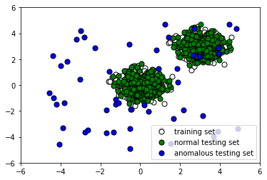
- Let's take a look at the data we have generated:
%matplotlib inline
import matplotlib.pyplot as plt

p1 = plt.scatter(X_train.x, X_train.y, c="white", s=50, edgecolor="black")
p2 = plt.scatter(X_test.x, X_test.y, c="green", s=50, edgecolor="black")
p3 = plt.scatter(X_outliers.x, X_outliers.y, c="blue", s=50, edgecolor="black")
plt.xlim((-6, 6))
plt.ylim((-6, 6))
plt.legend(
    [p1, p2, p3],
    ["training set", "normal testing set", "anomalous testing set"],
    loc="lower right",
)

plt.show()
The following screenshot shows the output:
- Now train an Isolation Forest model on our training data:
from sklearn.ensemble import IsolationForest

clf = IsolationForest()
clf.fit(X_train)
y_pred_train = clf.predict(X_train)
y_pred_test = clf.predict(X_test)
y_pred_outliers = clf.predict(X_outliers)
- Let's see how the algorithm performs. Append the labels to X_outliers:
X_outliers = X_outliers.assign(pred=y_pred_outliers)
X_outliers.head()
The following is the output:
| x | y | pred | |
|---|---|---|---|
| 0 | 3.947504 | 2.891003 | 1 |
| 1 | 0.413976 | -2.025841 | -1 |
| 2 | -2.644476 | -3.480783 | -1 |
| 3 | -0.518212 | -3.386443 | -1 |
| 4 | 2.977669 | 2.215355 | 1 |
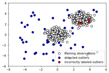
- Let's plot the Isolation Forest predictions on the outliers to see how many it caught:
p1 = plt.scatter(X_train.x, X_train.y, c="white", s=50, edgecolor="black")
p2 = plt.scatter(
    X_outliers.loc[X_outliers.pred == -1, ["x"]],
    X_outliers.loc[X_outliers.pred == -1, ["y"]],
    c="blue",
    s=50,
    edgecolor="black",
)
p3 = plt.scatter(
    X_outliers.loc[X_outliers.pred == 1, ["x"]],
    X_outliers.loc[X_outliers.pred == 1, ["y"]],
    c="red",
    s=50,
    edgecolor="black",
)

plt.xlim((-6, 6))
plt.ylim((-6, 6))
plt.legend(
    [p1, p2, p3],
    ["training observations", "detected outliers", "incorrectly labeled outliers"],
    loc="lower right",
)

plt.show()
The following screenshot shows the output:
- Now let's see how it performed on the normal testing data. Append the predicted label to X_test:
X_test = X_test.assign(pred=y_pred_test)
X_test.head()
The following is the output:
| x | y | pred | |
|---|---|---|---|
| 0 | 3.944575 | 3.866919 | -1 |
| 1 | 2.984853 | 3.142150 | 1 |
| 2 | 3.501735 | 2.168262 | 1 |
| 3 | 2.906300 | 3.233826 | 1 |
| 4 | 3.273225 | 3.261790 | 1 |
- Now let's plot the results to see whether our classifier labeled the normal testing data correctly:
p1 = plt.scatter(X_train.x, X_train.y, c="white", s=50, edgecolor="black")
p2 = plt.scatter(
    X_test.loc[X_test.pred == 1, ["x"]],
    X_test.loc[X_test.pred == 1, ["y"]],
    c="blue",
    s=50,
    edgecolor="black",
)
p3 = plt.scatter(
    X_test.loc[X_test.pred == -1, ["x"]],
    X_test.loc[X_test.pred == -1, ["y"]],
    c="red",
    s=50,
    edgecolor="black",
)

plt.xlim((-6, 6))
plt.ylim((-6, 6))
plt.legend(
    [p1, p2, p3],
    [
        "training observations",
        "correctly labeled test observations",
        "incorrectly labeled test observations",
    ],
    loc="lower right",
)

plt.show()
The following screenshot shows the output:
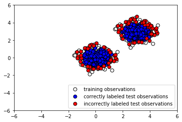
Evidently, our Isolation Forest model performed quite well at capturing the anomalous points. There were quite a few false negatives (instances where normal points were classified as outliers), but by tuning our model's parameters, we may be able to reduce these.
How it works...
The first step involves simply loading the necessary libraries that will allow us to manipulate data quickly and easily. In steps 2 and 3, we generate a training and testing set consisting of normal observations. These have the same distributions. In step 4, on the other hand, we generate the remainder of our testing set by creating outliers. This anomalous dataset has a different distribution from the training data and the rest of the testing data. Plotting our data, we see that some outlier points look indistinguishable from normal points (step 5). This guarantees that our classifier will have a significant percentage of misclassifications, due to the nature of the data, and we must keep this in mind when evaluating its performance. In step 6, we fit an instance of Isolation Forest with default parameters to the training data.
Note that the algorithm is fed no information about the anomalous data. We use our trained instance of Isolation Forest to predict whether the testing data is normal or anomalous, and similarly to predict whether the anomalous data is normal or anomalous. To examine how the algorithm performs, we append the predicted labels to X_outliers (step 7) and then plot the predictions of the Isolation Forest instance on the outliers (step 8). We see that it was able to capture most of the anomalies. Those that were incorrectly labeled were indistinguishable from normal observations. Next, in step 9, we append the predicted label to X_test in preparation for analysis and then plot the predictions of the Isolation Forest instance on the normal testing data (step 10). We see that it correctly labeled the majority of normal observations. At the same time, there was a significant number of incorrectly classified normal observations (shown in red).
Depending on how many false alarms we are willing to tolerate, we may need to fine-tune our classifier to reduce the number of false positives.