Search icon CANCEL
Subscription
0
Cart icon
Cart
Close icon
You have no products in your basket yet
Save more on your purchases!
Savings automatically calculated. No voucher code required
Arrow left icon
All Products
Best Sellers
New Releases
Books
Videos
Audiobooks
Learning Hub
Newsletters
Free Learning
Arrow right icon
Arrow up icon
GO TO TOP
Machine Learning for Cybersecurity Cookbook

You're reading from  Machine Learning for Cybersecurity Cookbook

Product type Book
Published in Nov 2019
Publisher Packt
ISBN-13 9781789614671
Pages 346 pages
Edition 1st Edition
Languages
Author (1):
Emmanuel Tsukerman Emmanuel Tsukerman
Profile icon Emmanuel Tsukerman
Toc

Table of Contents (11) Chapters close

Preface 1. Machine Learning for Cybersecurity 2. Machine Learning-Based Malware Detection 3. Advanced Malware Detection 4. Machine Learning for Social Engineering 5. Penetration Testing Using Machine Learning 6. Automatic Intrusion Detection 7. Securing and Attacking Data with Machine Learning 8. Secure and Private AI 9. Other Books You May Enjoy Appendix

Analyzing time series using statsmodels

A time series is a series of values obtained at successive times. For example, the price of the stock market sampled every minute forms a time series. In cybersecurity, time series analysis can be very handy for predicting a cyberattack, such as an insider employee exfiltrating data, or a group of hackers colluding in preparation for their next hit.

Let's look at several techniques for making predictions using time series.

Getting ready

Preparation for this recipe consists of installing the matplotlib, statsmodels, and scipy packages in pip. The command for this is as follows:

pip install matplotlib statsmodels scipy

How to do it...

In the following steps, we demonstrate several methods for making predictions using time series data:

  1. Begin by generating a time series:
from random import random

time_series = [2 * x + random() for x in range(1, 100)]
  1. Plot your data:
%matplotlib inline
import matplotlib.pyplot as plt

plt.plot(time_series)
plt.show()

The following screenshot shows the output:

  1. There is a large variety of techniques we can use to predict the consequent value of a time series:
    • Autoregression (AR):
from statsmodels.tsa.ar_model import AR

model = AR(time_series)
model_fit = model.fit()
y = model_fit.predict(len(time_series), len(time_series))
    • Moving average (MA):
from statsmodels.tsa.arima_model import ARMA

model = ARMA(time_series, order=(0, 1))
model_fit = model.fit(disp=False)
y = model_fit.predict(len(time_series), len(time_series))
    • Simple exponential smoothing (SES):
from statsmodels.tsa.holtwinters import SimpleExpSmoothing

model = SimpleExpSmoothing(time_series)
model_fit = model.fit()
y = model_fit.predict(len(time_series), len(time_series))

The resulting predictions are as follows:

How it works...

In the first step, we generate a simple toy time series. The series consists of values on a line sprinkled with some added noise. Next, we plot our time series in step 2. You can see that it is very close to a straight line and that a sensible prediction for the value of the time series at time  
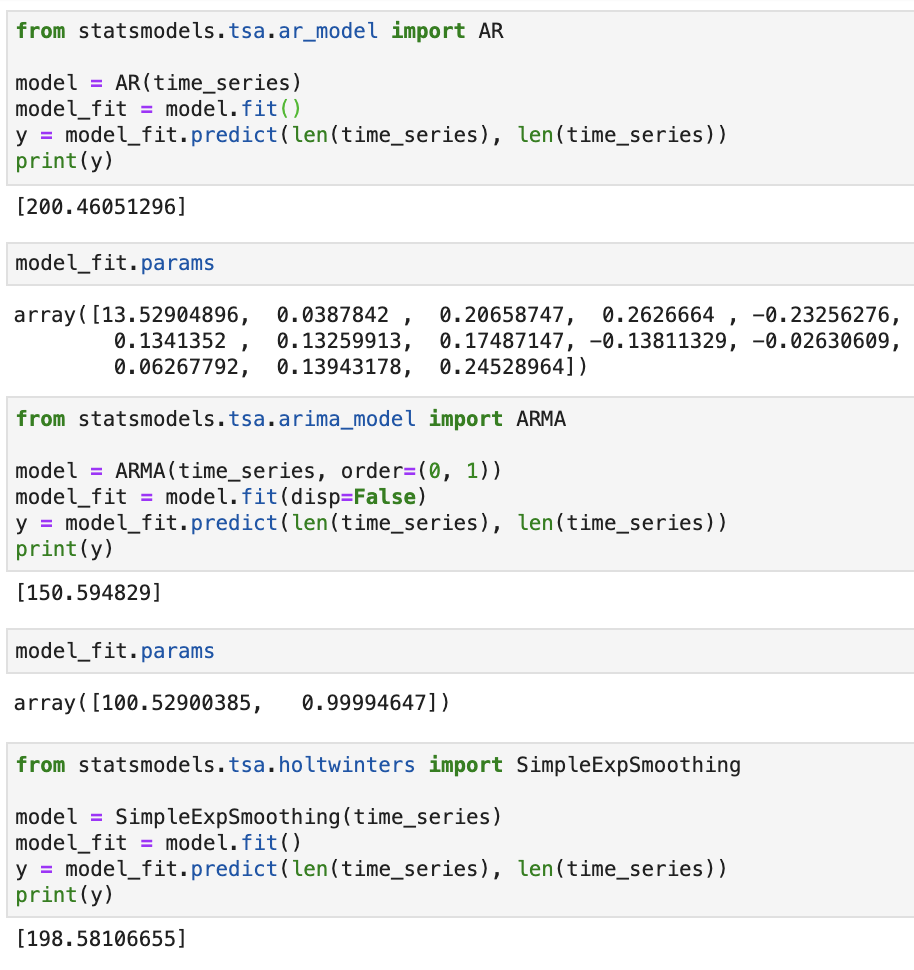
is . To create a forecast of the value of the time series, we consider three different schemes (step 3) for predicting the future values of the time series. In an autoregressive model, the basic idea is that the value of the time series at time t is a linear function of the values of the time series at the previous times. More precisely, there are some constants, , and a number, , such that:

As a hypothetical example, may be 3, meaning that the value of the time series can be easily computed from knowing its last 3 values.

In the moving-average model, the time series is modeled as fluctuating about a mean. More precisely, let be a sequence of i.i.d normal variables and let be a constant. Then, the time series is modeled by the following formula:

For that reason, it performs poorly in predicting the noisy linear time series we have generated.

Finally, in simple exponential smoothing, we propose a smoothing parameter, . Then, our model's estimate, , is computed from the following equations:

In other words, we keep track of an estimate, , and adjust it slightly using the current time series value, . How strongly the adjustment is made is regulated by the  parameter.

You have been reading a chapter from
Machine Learning for Cybersecurity Cookbook
Published in: Nov 2019 Publisher: Packt ISBN-13: 9781789614671
Register for a free Packt account to unlock a world of extra content!
A free Packt account unlocks extra newsletters, articles, discounted offers, and much more. Start advancing your knowledge today.
Unlock this book and the full library FREE for 7 days
Get unlimited access to 7000+ expert-authored eBooks and videos courses covering every tech area you can think of
Renews at $15.99/month. Cancel anytime