Standard explanation of autopilot decision trees
An SDC contains an autopilot that was designed with several artificial intelligence algorithms. Almost all AI algorithms can apply to an autopilot's need, such as clustering algorithms, regression, and classification. Reinforcement learning and deep learning provide many powerful calculations.
We will first build an autopilot decision tree for our SDC. The decision tree will be applied to a life and death decision-making process.
Let's start by first describing the dilemma from a machine learning algorithm's perspective.
The SDC autopilot dilemma
The decision tree we are going to create will be able to reproduce an SDC's autopilot trolley problem dilemma. We will adapt to the life and death dilemma in the Moral AI bias in self-driving cars section of this chapter.
The decision tree will have to decide if it stays in the right lane or swerves over to the left lane. We will restrict our experiment to four features:
f1: The security level on the right lane. If the value is high, it means that the light is green for the SDC and no unknown objects are on the road.f2: Limited security on the right lane. If the value is high, it means that no pedestrians might be trying to cross the street. If the value is low, pedestrians are on the street, or there is a risk they might try to cross.f3: Security on the left lane. If the value is high, it would be possible to change lanes by swerving over to the other side of the road and that no objects were detected on that lane.f4:Limited security on the left lane. If the value is low, it means that pedestrians might be trying to cross the street. If the value is high, pedestrians are not detected at that point.
Each feature has a probable value between 0 and 1. If the value is close to 1, the feature has a high probability of being true. For example, if f1 = 0.9, this means that the security of the right lane is high. If f1 = 0.1, this means that the security of the right lane is most probably low.
We will import 4,000 cases involving all four features and their 2 possible labeled outcomes:
- If
label = 0, the best option is to stay in the right lane - If
label = 1, the best option is to swerve to the left lane
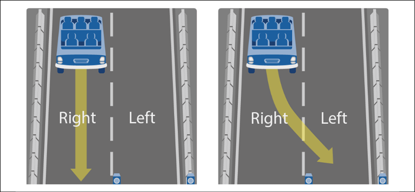
Figure 2.5: Autopilot lane changing situation
We will start by importing the modules required to run our decision tree and XAI.
Importing the modules
In this section, we will build a decision tree with the Google Colaboratory notebook. Go to Google Colaboratory, as explained in Chapter 1, Explaining Artificial Intelligence with Python. Open Explainable_AI_Decision_Trees.ipynb.
We will be using the following modules in Explainable_AI_Decision_Trees.ipynb:
numpyto analyze the structure of the decision treepandasfor data manipulationmatplotlib.pyplotto plot the decision tree and create an imagepickleto save and load the decision tree estimatorsklearn.treeto create the decision tree classifier and explore its structuresklearn.model_selectionto manage the training and testing datametricsis scikit-learn's metrics module and is used to measure the accuracy of the training processosfor the file path management of the dataset
Explainable_AI_Decision_Trees.ipynb starts by importing the modules mentioned earlier:
import numpy as np
import pandas as pd
import matplotlib.pyplot as plt
import pickle
from sklearn.tree import DecisionTreeClassifier, plot_tree
from sklearn.model_selection import train_test_split
from sklearn import metrics
import os
Now that the modules are imported, we can retrieve the dataset.
Retrieving the dataset
There are several ways to retrieve the dataset file, named autopilot_data.csv, which can be downloaded along with the code files of this chapter.
We will use the GitHub repository:
# @title Importing data <br>
# Set repository to "github"(default) to read the data
# from GitHub <br>
# Set repository to "google" to read the data
# from Google {display-mode: "form"}
import os
from google.colab import drive
# Set repository to "github" to read the data from GitHub
# Set repository to "google" to read the data from Google
repository = "github"
if repository == "github":
  !curl -L https://raw.githubusercontent.com/PacktPublishing/Hands-On-Explainable-AI-XAI-with-Python/master/Chapter02/autopilot_data.csv --output "autopilot_data.csv"
  # Setting the path for each file
  ip = "/content/autopilot_data.csv"
  print(ip)
The path of the dataset file will be displayed:
/content/autopilot_data.csv
Google Drive can also be activated to retrieve the data. The dataset file is now imported. We will now process it.
Reading and splitting the data
We defined the features in the introduction of this section. f1 and f2 are the probable values of the security on the right lane. f3 and f4 are the probable values of the security on the left lane. If the label is 0, then the recommendation is to stay in the right lane. If the label is 1, then the recommendation is to swerve over to the left lane.
The file does not contain headers. We first define the names of the columns:
col_names = ['f1', 'f2', 'f3', 'f4', 'label']
We will now load the dataset:
# load dataset
pima = pd.read_csv(ip, header=None, names=col_names)
print(pima.head())
We can now see that the output is displayed as:
     f1    f2    f3    f4  label
0  0.51  0.41  0.21  0.41      0
1  0.11  0.31  0.91  0.11      1
2  1.02  0.51  0.61  0.11      0
3  0.41  0.61  1.02  0.61      1
4  1.02  0.91  0.41  0.31      0
We will split the dataset into the features and target variable to train the decision tree:
# split dataset in features and target variable
feature_cols = ['f1', 'f2', 'f3', 'f4']
X = pima[feature_cols] # Features
y = pima.label # Target variable
print(X)
print(y)
The output of X is now stripped of the label:
        f1    f2    f3    f4
0     0.51  0.41  0.21  0.41
1     0.11  0.31  0.91  0.11
2     1.02  0.51  0.61  0.11
3     0.41  0.61  1.02  0.61
4     1.02  0.91  0.41  0.31
...    ...   ...   ...   ...
3995  0.31  0.11  0.71  0.41
3996  0.21  0.71  0.71  1.02
3997  0.41  0.11  0.31  0.51
3998  0.31  0.71  0.61  1.02
3999  0.91  0.41  0.11  0.31
The output of y only contains labels:
0       0
1       1
2       0
3       1
4       0
       ..
3995    1
3996    1
3997    1
3998    1
3999    0
Now that we have separated the features from their labels, we are ready to split the dataset. The dataset is split into training data to train the decision tree and testing data to measure the accuracy of the training process:
# Split dataset into training set and test set
X_train, X_test, y_train, y_test = train_test_split(X, y,
    test_size=0.3, random_state=1) # 70% training and 30% test
Before creating the decision tree classifier, let's explore a theoretical description.
Theoretical description of decision tree classifiers
The decision tree in this chapter uses Gini impurity values to classify the features of the record in a dataset node by node. The nodes at the top of the decision tree contain the highest values of Gini impurity.
In this section, we will take the example of classifying features into the left lane or right lane labels. For example, if the Gini value is <=0.46 for feature 4, f4, then the child node on the left filters the true values, which will favor keeping the SDC on the right lane. The child node on the right is false for the f4 condition and will favor sending the SDC on the left lane:
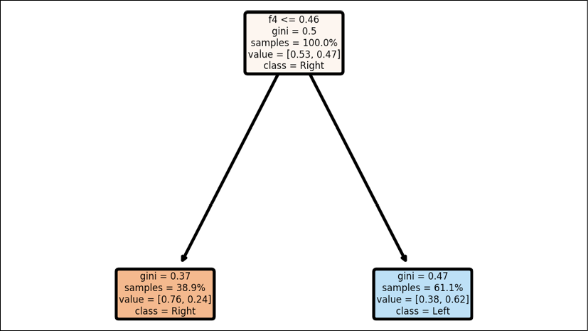
Figure 2.6: Decision tree
Let k represent the probability of a data point being incorrectly classified. Let X represent the dataset we are applying the decision tree to.
The equation of Gini impurity calculates the probability of each feature occurring and multiplies the result by 1, that is, the probability of occurring on the remaining values, as shown in the following equation:

The decision train is built on the gain of information on the features that contain the highest Gini impurity value.
As the decision tree classifier calculates the Gini impurity at each node and creates child nodes, the decision tree's depth increases, as shown in the following graph:
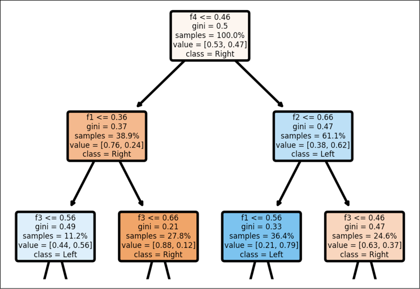
Figure 2.7: Structure of a decision tree
You can see examples of the whole structure of the process in the XAI section of this chapter, XAI applied to an autopilot decision tree.
With these concepts in mind, let's create a default decision tree classifier.
Creating the default decision tree classifier
In this section, we will create the decision tree classifier using default values. We will explore the options in the XAI applied to an autopilot decision tree section of this chapter.
A decision tree classifier is an estimator. An estimator is any ML algorithm that contains learning functions. A classifier will classify the data.
The default decision tree classifier can be created with a single line:
# Create decision tree classifier object
# Default approach
estimator = DecisionTreeClassifier()
print(estimator)
The following program displays the default values of the classifier:
DecisionTreeClassifier(ccp_alpha=0.0, class_weight=None,
                       criterion='gini', max_depth=None,
                       max_features=None, max_leaf_nodes=None,
                       min_impurity_decrease=0.0,
                       min_impurity_split=None, min_samples_leaf=1,
                       min_samples_split=2,
                       min_weight_fraction_leaf=0.0,
                       presort='deprecated', random_state=None,
                       splitter='best')
We will go into more detail in the XAI applied to an autopilot decision tree section of this chapter. At this point, we will note the three key options:
criterion='gini': We are applying the Gini impurity algorithm described earlier.max_depth=None: There is no maximum depth that constricts the decision tree, which maximizes its size.min_impurity_split=None: There is no minimum impurity split, which means that even small values will be taken into account. There is no constraint on expanding the size of a decision tree.
We can now train, measure, and save the model of the decision tree classifier.
Training, measuring, and saving the model
We have loaded and split the data into training data and testing data. We have created a default decision tree classifier. We can now run the training process with our training data:
# Train decision tree classifier
estimator = estimator.fit(X_train, y_train)
Once the training is over, we want to test the trained model using our test data. The estimator will make predictions:
# Predict the response for the test dataset
print("prediction")
y_pred = estimator.predict(X_test)
print(y_pred)
The output will display the predictions:
prediction
[0 0 1 ... 1 1 0]
The problem we face here is that we have no idea how accurate the predictions were by just looking at them. We need a measurement tool. In the XAI applied to an autopilot decision tree section of this chapter, we will be using our own measurement tool. We will need a customized measurement tool to check whether the predictions are biased or not, ethical or not, and legal or not. In this section, we will use the standard metrics function provided by scikit-learn:
# Model accuracy
print("Accuracy:", metrics.accuracy_score(y_test, y_pred))
The output is displayed:
Accuracy: 1.0
The technical accuracy is perfect, as we can see. However, we do not know if one of the predictions is to stay on a lane and kill one or several pedestrians or not! We will need more explainability control, as we will discuss in the XAI applied to an autopilot decision tree section of this chapter. In that section, we will learn how to deactivate a model with an alert when necessary.
We will now save the model. This does not seem that important from a technical standpoint. After all, we are just saving the parameters of the model so that it will make decisions without needing to be trained again.
From a moral, ethical, and legal standpoint, we have just signed our legal accountability contract. If a fatal accident occurs, the legal experts will take this model apart and ask for explanations. The model is saved with the following code:
# save model
pickle.dump(estimator, open("dt.sav", 'wb'))
To check whether the model has been saved, click on the Files button on the left of the Google Colaboratory page:

Figure 2.8: Colab file manager
You should see dt.sav in the list of files displayed:

Figure 2.9: Saving the test data
We have trained, tested, and saved our model. We can now display our decision tree.
Displaying a decision tree
A graph of a decision tree is an excellent tool for XAI. However, in many cases, the number of nodes displayed will only confuse a user or even a developer. In this section, we will focus on a default model. We will customize the decision tree graph in the XAI applied to an autopilot decision tree section. In this section, we will first learn how to implement a default model.
The program first imports the figure module of matplotlib:
from matplotlib.pyplot import figure
Now we can create the figure using two basic options:
plt.figure(dpi=400, edgecolor="r", figsize=(10, 10))
dpi will determine the dots per inch of your graph. It does not seem that important to pay attention to this option. However, it is a critical option because it's a trial and error process. Large decision trees produce large graphs that make them difficult to see in detail. The nodes might be too small to understand and visualize even when zooming in. If dpi is too small when the graph is large, you won't see anything. If dpi is too large when the graph is small, your nodes will spread out and make it difficult to see them as well.
Both figsize and dpi are related, and, as such, figsize will produce the same effects as dpi when you adjust the size of the graph.
You can overcome this problem with a trained model, and if the datasets are homogeneous, you can try different values of figsize and dpi until you find the ones that fit your needs.
We will now define the name of the labels of our features in an array:
F = ["f1", "f2", "f3", "f4"]
We also want to visualize the class of each node:
C = ["Right", "Left"]
We are now ready to use the plot_tree function imported from scikit-learn:
plot_tree(estimator, filled=True, feature_names=F, rounded=True,
          precision=2, fontsize=3, proportion=True, max_depth=None,
          class_names=C)
We have used several options provided by plot_tree:
estimator: Contains the name of the estimator of the decision tree.filled=True: Fills the nodes with the color of their class.feature_names=F: Contains the labels of the feature array.rounded=True: Rounds the borders of the nodes.precision=2: The number of digits displayed for Gini impurity.fontsize=3: Must be adapted to the graph likefigsizeanddpi.proportion=True: WhenTrue, the values will be proportions and percentages.max_depth=None: Limits the maximum depth of the graph.Nonedisplays the whole graph.class_names=C: Contains the labels of the class array.
The program saves the figure:
plt.savefig('dt.png')
You can open this image. Click on the Files button on the left of the Google Colaboratory page:

Figure 2.10: File manager
You should see dt.png in the list of files displayed:

Figure 2.11: File upload
You can click on the name of the image and open it. You can also download it.
The image is also displayed underneath the cell with the following code:
plt.show()
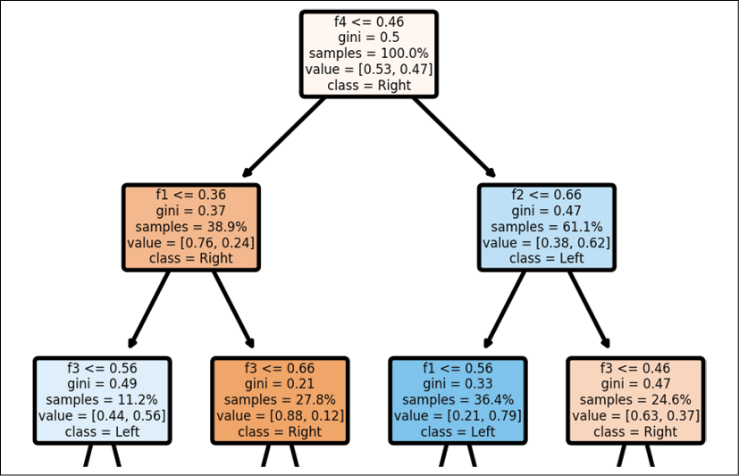
Figure 2.12: Decision tree structure
The decision tree structure shows the path a decision takes depending on its value as expected.
In this section, we imported the autopilot dataset and split it to obtain training data and test data. We then created a decision tree classifier with default options, trained it, and saved the model. We finally displayed the graph of the decision tree.
We now have a default decision tree classifier. We now need to work on our explanations when the decision tree faces life and death situations.


