Search icon CANCEL
Subscription
0
Cart icon
Your Cart (0 item)
Close icon
You have no products in your basket yet
Save more on your purchases! discount-offer-chevron-icon
Savings automatically calculated. No voucher code required.
Arrow left icon
Explore Products
Best Sellers
New Releases
Books
Videos
Audiobooks
Learning Hub
Newsletter Hub
Free Learning
Arrow right icon
timer SALE ENDS IN
0 Days
:
00 Hours
:
00 Minutes
:
00 Seconds
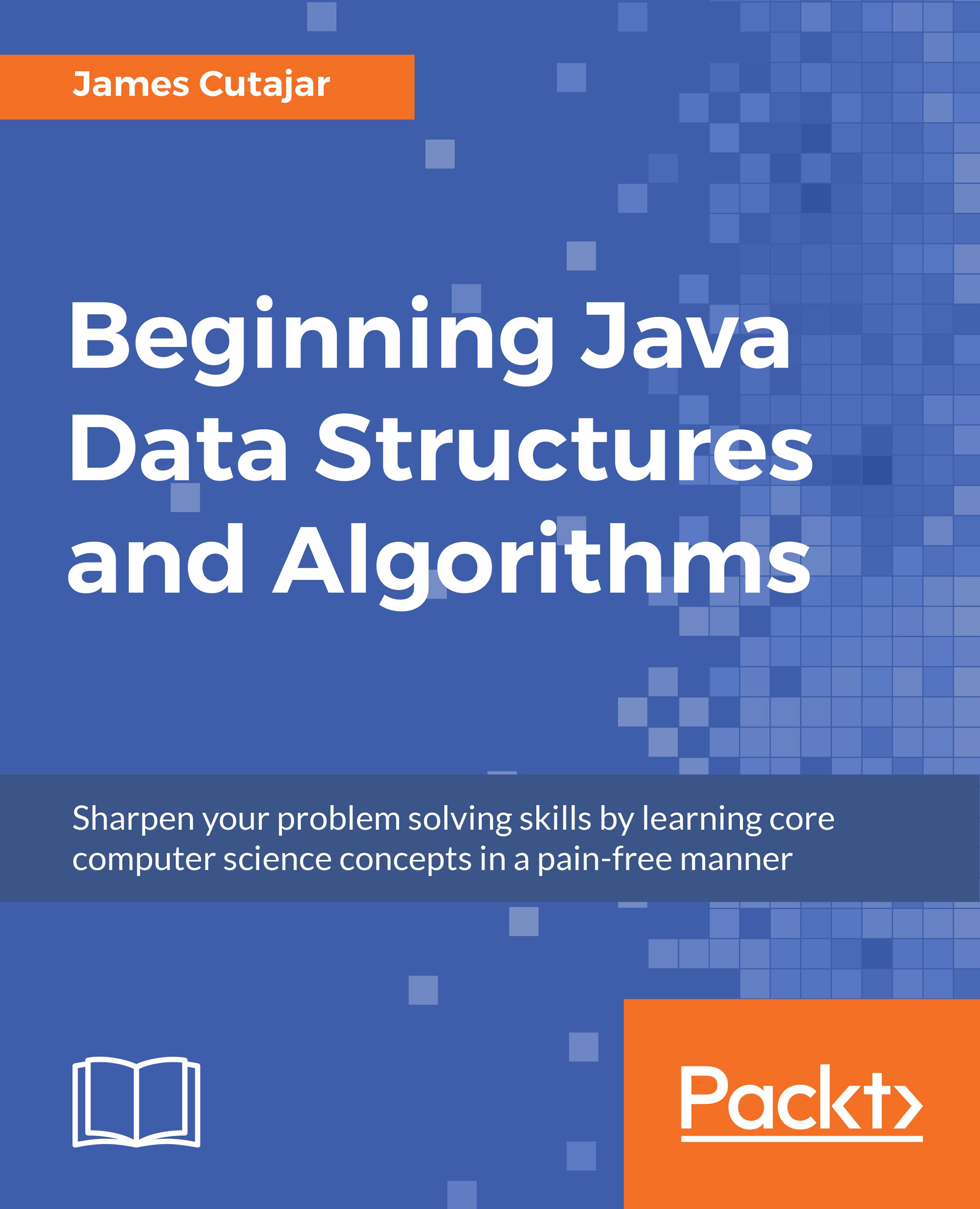
Beginning Java Data Structures and Algorithms

Beginning Java Data Structures and Algorithms: Sharpen your problem solving skills by learning core computer science concepts in a pain-free manner

eBook
€8.99 €16.99
Paperback
€20.99
Subscription
Free Trial
Renews at €18.99p/m

What do you get with Print?

Product feature icon Instant access to your digital eBook copy whilst your Print order is Shipped
Product feature icon Paperback book shipped to your preferred address
Product feature icon Download this book in EPUB and PDF formats
Product feature icon Access this title in our online reader with advanced features
Product feature icon DRM FREE - Read whenever, wherever and however you want
OR
Modal Close icon
Payment Processing...
tick Completed

Shipping Address

Billing Address

Shipping Methods
Table of content icon View table of contents Preview book icon Preview Book

Beginning Java Data Structures and Algorithms

Algorithms and Complexities

An algorithm is a set of logical instructions to perform a particular task. Algorithms are everywhere nowadays. As a software developer, understanding the core principles of algorithms and data structures will enable you to make informed decisions on how to approach a particular problem. This is valid whether you're working in a bank writing accounting software or doing medical research data, mining genetic code. How do we determine which is the right algorithm to use when more than one solution to a problem exists? In this chapter, we will examine different types of algorithms and discuss how the performance varies in each. We will discuss what makes an algorithm more efficient than another and how to express the complexity of each.

The common examples of algorithms include traffic lights regulating congestion on the streets, face recognition software on smartphones, recommendation technologies, and so on.
It's important for you to understand that an algorithm is just a small part of an application used to solve a well-defined problem. Examples such as sorting a list of numbers, finding the shortest route, or word prediction are all correct. Big software applications, such as email clients or an operating system are improper examples.

By the end of this chapter, you will be able to:

  • Define an algorithm with an example
  • Measure algorithmic complexity
  • Identify algorithms with different complexities
  • Assess various examples with different runtime complexities

Developing Our First Algorithm

An algorithm can be seen as a roadmap or a set of instructions to accomplish a well-defined task. In this section, we will build a simple example of one such algorithm to help us get started.

Algorithm for Converting Binary Numbers to Decimal

Number systems have different bases. Decimals numbers with a base of ten are what most of us are familiar with. Computers, on the other hand, use only ones and zeros (binary). Let's try to write some code that converts binary numbers to decimals.

Specifically, we want to develop an algorithm that accepts a string containing ones and zeros and returns an integer.

We can convert the binary string by following these steps:

  1. Start from the end of the string and process each character at a time. The position of each digit in the binary string corresponds to a decimal number in a sequence.
  2. To generate this sequence, you start from one and multiply by two every time, so one, two, four, eight, and so on (see Conversion Sequence row of Table 1.1). More formally, the sequence is a geometric progression that starts at one and progresses in a common ratio of two.
  3. We then apply the binary string as a mask on this sequence (see the Binary String (Mask) row of Table 1.1).
  4. The result is a new sequence where the values are only kept if the corresponding position in the binary string has a value of one (see the Result row of Table 1.1).
  5. After applying the mask, we just need to sum up the resulting numbers together.
Conversion Sequence 16 8 4 2 1
Binary String (Mask) 1 0 1 1 0
Result 16 0 4 2 0
Table 1.1: Binary to decimal masking

In the preceding example (Table 1.1), resulting total is 22. This is our decimal number corresponding to the binary number 10110.

To design our algorithm, it's important to realize that we don't need to store the entire conversion sequence. Since we are processing one binary digit at a time (starting from the back), we only need to use the conversion number corresponding to the binary position we are processing.

Snippet 1.1 shows us how we can do this. We use a single conversion variable instead of a sequence and initialize this variable to the value of one. We then use a loop to iterate over the length of the binary string starting from the end. While iterating, if the digit at our current position is one, we add the current conversion variable to the final result. We then simply double the current conversion variable and repeat. The code snippet is as follows:

public int convertToDecimal(String binary) {
int conversion = 1;
int result = 0;
for (int i = 1; i <= binary.length(); i++) {
if (binary.charAt(binary.length() - i) == '1')
result += conversion;
conversion *= 2;
}
return result;
}
Snippet 1.1: Binary to decimal. Source class name: BinaryToDecimal.

Go to
https://goo.gl/rETLfq to access the code.

Activity: Writing an Algorithm to Convert Numbers from Octal To Decimal

Scenario

In aviation, the aircraft's transponders transmit a code so that they can identify one another. This code uses the octal system, a number system which has a base of 8. We have been asked to write a method to convert octal numbers into decimals. For example, the octal number 17 is represented as 15 in the decimal system.

Aim

To be able to adapt the algorithm shown in the previous section to be used in a different scenario.

Prerequisites

  • Ensure that you have a class available on the following path:

https://github.com/TrainingByPackt/Data-Structures-and-Algorithms-in-Java/blob/master/src/main/java/com/packt/datastructuresandalg/lesson1/activity/octaltodecimal/OctalToDecimal.java

  • You will find the following method that needs implementing:
 public int convertToDecimal (String octal) 
  • If you have your project set up, you can run the unit test for this activity by running the following command: 
gradlew test --tests com.packt.datastructuresandalg.
lesson1.activity.octaltodecimal*

Steps for Completion

  1. The algorithms shown in Snippet 1.1 the preceding snippets of code can be adapted to work with octal numbers instead of binary.
  2. Change the base from two to eight. This can be done by changing the conversion multiplier variable in Snippet 1.1.
  3. Parse the digit being processed to convert it into an integer. This integer can then be multiplied by the conversion variable or result of the power function.

In this first section, we introduced the idea of algorithms by working on a simple example. It's important to note that for every problem multiple solutions exist. Choosing the right algorithm to solve your problem will depend on several metrics, such as performance and memory requirements.

Measuring Algorithmic Complexity with Big O Notation

Algorithmic complexity is a way to describe the efficiency of an algorithm as a relation of its input. It can be used to describe various properties of our code, such as runtime speed or memory requirements. It's also a very important tool programmers should understand to write efficient software. In this section, we will start by describing a scenario, introducing the section, and then dive into the details of the various types of complexities and the different techniques to measure them.

Complexity Example

Imagine we were given the task of writing a piece of software for air traffic control. Specifically, we were asked to write an algorithm that, in a pre-defined space and altitude, will ring out an alarm if any two aircraft get too close to each other.

In our implementation, we solved the problem by computing all possible distances between every pair in our airspace and keeping only the minimum distance. If this minimum distance is less than a certain threshold, our software will ring out an alarm. The following snippet of code shows this solution:

public double minimumDistance(List<Point> allPlanes) {
double minDistance = Double.MAX_VALUE;
for (Point p1 : allPlanes) {
for (Point p2 : allPlanes) {
double d = p1.distanceTo(p2);
if (d != 0 && d < minDistance) minDistance = d;
}
}
return minDistance;
}
Snippet 1.2: Minimum distance. Source class name: ClosestPlane and Point.

Note that the Point class in the preceding piece of code is not shown. Go to
https://goo.gl/iDHD5J to access the code.

Our little algorithm works fine for a couple of years and the controllers are happy to have this useful alerting. However, over the years, air traffic increases at a fast rate, and instead of having to monitor a few hundred aircraft at any given time, our algorithm has to handle tens of thousands of points. At busy times, the software is having trouble keeping up with the increased load.

We are called in to investigate and we start to write some benchmarks to test how fast the algorithm performs. We obtain the timings shown in Table 1.2. As you can see, we are doubling the load on every run; however, our algorithm is not scaling up in the same manner. Our algorithm is not slowing down at the same rate as our input.

Intuitively, you may expect that if you double the number of planes, the algorithm has, then you have twice the amount of work to do, and as a result, it should take twice as long. However, this is not what is happening.

When we double the number of planes, the time taken doesn't just double but skyrockets.

For example, our algorithm takes 2.6 seconds (2,647 ms) to finish when it's dealing with 16,000 planes. However, if we double the amount of planes to 32,000, the time it takes increases to 10.4 seconds (10,488 ms), a four-fold increase!

Number of planes Time taken (ms)
1000 27
2000 48
4000 190
8000 664
16000 2647
32000 10488


In the following graph, we plot the benchmark results in a chart. What is going on here? Our algorithm is doing a lot of work due to the nested loop. For every plane point in its input, it's calculating the distance to every other plane. This results in n2 calculations, where n is the number of planes we are monitoring. We can say that our algorithm has a runtime performance of O(n2), read as big O of n squared. Alternatively, we can also call it the quadratic runtime performance. Take a look at this graph:

Figure 1.1: Algorithm benchmark result plot

The algorithm listed in Snippet 1.2 is a slow solution for the closest pair problem. There exists a much more efficient solution that involves a divide and conquer technique.

This class of algorithms is explored in detail in the second part of this book in Chapter 4, Algorithm Design Paradigms, where we present a faster solution to the closest pair problem.

Increasing the input load on your code does not always mean that the resource consumption will also increase in a directly proportional manner. The relation between the input size of your problem and resource usage (CPU time, memory, and so on) is what this section is all about.

In the next section, we will see different types of these relations between the problem, input size, and resource usage.

Understanding Complexity

To better understand algorithmic complexity, we can make use of an analogy. Imagine that we were to set different types of algorithms so that they compete against one another on a race track. However, there is a slight twist: The race course has no finish line.

Since the race is infinite, the aim of the race is to surpass the other, slower opponents over time and not to finish first. In this analogy, the race track distance is our algorithm input. How far from the start we get, after a certain amount of time, represents the amount of work done by our code.

Recall the quadratic method for measuring the closest pair of planes in the preceding section. In our fictitious race, the quadratic algorithm starts quite fast and is able to move quite a distance before it starts slowing down, similar to a runner that is getting tired and slowing down. The further it gets away from the start line, the slower it gets, although it never stops moving.

Not only do the algorithms progress through the race at different speeds, but their way of moving varies from one type to another. We already mentioned that O(n2) solutions slow down as they progress along the race. How does this compare to the others?

Another type of runner taking part in our imaginary race is the linear algorithm. Linear algorithms are described with the notation of O(n). Their speed on our race track is constant. Think of them as an old, reliable car moving at the same fixed speed.

In real life, solutions that have an O(n) runtime complexity have a running performance that is directly proportional to the size of their input. 

This means, for example, that if you double the input size of a linear algorithm, the algorithm would also take about twice as long to finish.

The efficiency of each algorithm is always evaluated in the long run. Given a big enough input, a linear algorithm will always perform better than a quadratic one.

We can go much quicker than O(n). Imagine that our algorithm is continually accelerating along the track instead of moving constantly. This is the opposite of quadratic runtime. Given enough distance, these solutions can get really fast. We say that these type of algorithms have a logarithmic complexity written as O(log n).

In real life, this means that the algorithm doesn't slow much as the size of the input increases. Again, it doesn't matter if at the start, the algorithm performs slower than a linear one for a small input, as for a big enough input, a logarithmic solution will always outperform the linear one.

Can we go even faster? It turns out that there is another complexity class of algorithms that performs even better.

Picture a runner in our race who has the ability to teleport in constant time to any location along our infinite track. Even if the teleportation takes a long time, as long as it's constant and doesn't depend on the distance traveled, this type of runner will always beat any other. No matter how long the teleportation takes, given enough distance, the algorithm will always arrive there first. This is what is known as a constant runtime complexity, written as O(1). Solutions that belong to this complexity class will have a runtime independent of the input size given.

On the other side of the spectrum, we can find algorithms that are much slower than quadratic ones. Complexities such as cubic with O(n3) or quartic with O(n4) are examples. All of the mentioned complexities up to this point are said to be polynomial complexities.

A polynomial is simply a mathematical term used for expressions. Expressions such as 3x5 + 2x3 + 6, 2x – 3, or even just 5 are all good examples. The key here is that polynomial complexities are of the form O(nk), where k is a positive, non-fractional constant.

Not all solutions have a polynomial time behavior. A particular class of algorithms scale really badly in proportion to their input with a runtime performance of O(kn). In this class, the efficiency degrades exponentially with the input size. All the other types of polynomial algorithms will outperform any exponential one pretty fast. Figure 1.2 shows how this type of behavior compares with the previously mentioned polynomial algorithms.

The following graph also shows how fast an exponential algorithm degrades with input size:
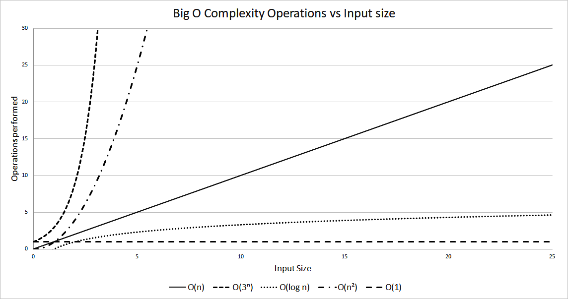
Figure 1.2: Operations performed versus input size for different algorithms

How much faster does a logarithmic algorithm perform versus a quadratic one? Let's try to pick a particular example. A specific algorithm performs about two operations to solve a problem; however, the relation to its input is O(n2).

Assuming each operation is a slow one (such as file access) and has a constant time of about 0.25 milliseconds, the time required to perform those operations will be as shown in Table 1.3. We work out the timings by Time = 0.25 * operations * n2, where operations is the number of operations performed (in this example it's equal to 2), n is the input size, and 0.25 is the time taken per operation:

Input Size (n) Time: 2 operations O(n2) Time: 400 operations O(log n)
10 50 milliseconds 100 milliseconds
100 5 seconds 200 milliseconds
1000 8.3 minutes 300 milliseconds
10000 13.8 hours 400 milliseconds
Table 1.3: How fast does it run?

Our logarithmic algorithm performs around 400 operations; however, its relation to the input size is logarithmic. Although this algorithm is slower for a smaller input, it quickly overtakes the quadratic algorithm. You can notice that, with a large enough input, the difference in performance is huge. In this case, we work out the timing using Time = 0.25 * operations * log n, with operations = 400.

Activity: Developing a Timing Table Using the Exponential Algorithm

Scenario

We have been asked to develop a timing table using an input size of 2, 10, 30, and 50 for an exponential algorithm of O(2n). Assume an operation time of 0.5 ms and that the algorithm only performs one operation.

Aim

To discover how badly exponential algorithms scale.

Steps for Completion

  1. 0.5 x 22 = 2 ms
  2. 0.5 x 210 = 512 ms
  3. 0.5 x 230 = 0.536 billion ms = 6.2 days
  4. 0.5 x 250 = 5.629 and 1014 ms = 17838 years

Output

The results may be as follows:

Input Size (n) Time : 1 Operations O(2n)
2 2 milliseconds
10 512 milliseconds
30 6.2 days
50 17838 years
Table 1.4: Timings for the O(2n) algorithm

In this section, we have compared different types of algorithmic runtime complexities. We have seen how each compares against the others, starting from the theory's fastest of O(1) to some of the slowest with O(kn). It's also important to understand that there is a difference between theory and practice. For example, in real life, a quadratic algorithm may outperform a linear one if the operations performed are less, the input is a fixed size, and is small.

Complexity Notation

In the previous section, we have seen how we can use the big O notation to measure the runtime performance to our algorithms in proportion to the input size. We have neither examined in detail what O(n) really means nor have we considered the performance of our algorithm in relation to the type of input it's given.

Consider the following code snippet. The method accepts an array containing a string and searches for a match. If one is found, the index of the array is returned. We will use this example and try to measure the runtime complexity. The code is as follows:

public int search(String strToMatch, String[] strArray) {
for (int i = 0; i < strArray.length; i++) {
if (strArray[i].equals(strToMatch)) {
return i;
}
}
return -1;
}
Snippet 1.3: Array search. Source class name: ArraySearch.

Go to
https://goo.gl/egw1Sn to access the code. 

There are a number of operations happening inside the loop. The obvious ones are the arrays accessing at i and the string equals. However, we also have the increment of i, the assignment of the new incremented value to i and the comparison of i being less than the length of the array. However, this is not the end of the story. The equals() method is also matching each character of the string to an element at i in the array.

The following table lists all these operations:

Operation name Code Count
Array access strArray[i] 1
String equality .equals(strToMatch) String length
Array pointer increment and assignment i = i + 1 2
Reading array length and comparing to pointer i < strArray.length 2
Table 1.5: Operations performed in the ArraySearch method for every item

We have seen that for each processed item in the search array, we perform 5 + m operations, where m is the length of the search string. The next aspect to look at is to work out how often we perform this. The number of times we perform the operations mentioned in Table 1.5 doesn't just rely on the length of our input; it also depends on how quick we are in finding our match in the input array, that is, it depends on the actual array's contents.

The best case of an algorithm is when the input causes the algorithm to perform in the most efficient manner possible. The worst case is the opposite, which is when a particular input makes it behave in the least efficient manner possible.

If we are lucky and the item we are searching for is located in the first element of the search array, we perform only 5 + m operations. This is the best case and is the fastest manner our search can compute.

The worst case of this algorithm is either when our item is at the end of the array or when the item is not found at all. Both of these scenarios will have us then check the entire contents of the array. In the worst case, we end up performing n(5 + m) operations, where n is the array size.

In this example, we can say that the worst-case runtime complexity for our algorithm is O(mn) and our best case, when our algorithm finds a match immediately, is O(m). We will see in the following sub-section how we arrive at this result from 5 + m and n(5 + m).

Another algorithmic analysis that is commonly used is the average case performance. The average case complexity can be found by averaging the performance over all possible inputs. This is useful, as in certain scenarios, the worst case has a low chance of occurring.

Although we have the best, average, and worst-case complexities, the worst case is usually the most used when measuring and comparing different algorithms to one another. Apart from runtime performance, the other most common use of big O notation is to measure memory requirements. However, it can be used for any resource, such as disk space or network usage.

Identifying the Best and Worst Performance of an Algorithm While Checking for Duplicates in an Array

We want to determine the complexity of an algorithm checking for duplicates in an array by considering the best and worst case performance. Find the number of operations performed in the Snippet 1.4 for both the worst and best case. There is no need to work out the algorithmic complexity in big O notation. Assume that the inner loop results in eight operations every time it executes.

For the outer loop, assume four operations:

public boolean containsDuplicates(int[] numbers) {
for (int i=0; i<numbers.length; i++) {
for (int j=0; j<numbers.length; j++) {
if (i != j && numbers[i] == numbers[j]) return true;
}
}
return false;
}
Snippet 1.4: Checking for duplicates. Source class name: Duplicates.

Go to
https://goo.gl/wEUqYk to access the code.

To do this, we should perform the following steps:

  1. In the worst- case, we execute the inner loop n times (array length).
  2. In the best case, we only execute the inner loop only twice.
  3. The best case is when the duplicate numbers are in the front of the input array. The worst is when the array doesn't contain any duplicates.
  1. The worst case is when the array doesn't contain duplicates and is of size n:
    • For the outer loop, we have 4*n operations
    • For the inner loop, we have n*(n*8) operations
    • In total, we have 4n + 8n2 operations
  2. In the best case, the duplicates are the first two items in the array:
    • For the outer loop, we have 4 operations
    • For the inner loop, we have 2*8 operations as the inner loop executes twice to get to the second item in the array where the duplicate is located
    • In total, we have 20 operations

We have seen how we can analyze the number of operations performed in an algorithm and how we can use big O notation to describe the best and worst case. We also discussed how the notation can be used to describe any resource usage. In the next section, we'll describe some basic rules that are used when using the notation.

Notation Rules

There are two simple rules to follow when we want to express an algorithm using the big O notation. In this section, we will understand how to convert the expression from 4n + 8n2 to the big O notation equivalent.

The first rule to follow is to drop any constants.

For example, 3n + 4 becomes n and, a single constant such as 5 becomes 1. If an algorithm simply has 4 constant instructions that don't depend on the input, we say the algorithm is O(1), also known as constant time complexity.

The second rule is to drop everything except the highest order.

To understand why we adopt the second rule, it's important to realize that for a large value of n, anything but the highest order becomes irrelevant. When we have a large enough input, the performance difference is negligible.

Consider an algorithm that performs n + n2 + n3. The highest order variable of this is the n3 part. If we keep the highest order, we end up with a big O runtime complexity of O(n3).

Activity: Converting Expressions to Big O Notations

Scenario

To convert the expression 3mn + 5mn+2n+ 6 to a big O notation, firstly we drop any constants from the expression, leaving us with mn+mn4+n2. Next, we simply keep the highest order part, which results in O(mn4).

For each of the expressions found in Table 1.6, find the equivalent in big O notation:

Expression 3mn 5n + 44n2 + 4 4 + 5 log n 3n + 5n2 + 8
Table 1.6: Find big O equivalent

Aim

To apply notation rules to convert expressions into big O notations.

Steps for completion

  1. Identify and drop the constants in the expression:
    • 3mn → No constants → 3mn
    • 5n + 44n2 + 4 → → 5n + 44n2
    • 4 + 5 log n → → 5 log n
    • 3n + 5n2 + 8 → → 3n + 5n2
  2. Drop everything except the highest-order part:
    • 3mn → O(mn)
    • 5n + 44n→ O(n2)
    • 5 log n → O(log n)
    • 3n + 5n→ O(3n)

Output

The outcome may be as follows:

Expression 3mn

5n + 44n2 + 4

4 + 5 log n 3n + 5n2 + 8
Solution O(mn) O(n2) O(log n) O(3n)
Table 1.7: Solution to find big O equivalent activity

In this section, we have explored two simple rules used for converting expressions to big O notations. We have also learned why we keep only the highest-order from the expression. In the next section, we shall see some examples of algorithms with different complexities.

Identifying Algorithms with Different Complexities

In this section, we shall look into examples of different complexities. This is important so that we can learn to recognize algorithms that belong to different complexity classes and possibly attempt improving the performance of each.

Figuring out the worst case complexity can be quite difficult for some algorithms. Sometimes, this requires some experience and is best learned by looking at many examples and getting familiar with different types of algorithms.

Linear Complexity

Linear algorithms are the ones where the work done varies in direct proportion with the input size, that is, if you double the input size, you double the work done. These typically involve a single pass through the input.

The problem presented in this example is that of counting the number of occurrences of a particular character in a string. Imagine we are given the string Sally sells sea shells on the seashore, and we want to find out the number of occurrences of the letter a.

The following code in Snippet 1.5 goes through each character in the input string and if the character at the current position matches the search letter, a counter is increased. At the end of the loop, the final count is returned. The code is as follows:

public int countChars(char c, String str) {
int count = 0;
for (int i = 0; i < str.length(); i++) {
if (str.charAt(i) == c) count++;
}
return count;
}
Snippet 1.5: Count the number of characters in a string. Source class name: CountChars.

Go to
https://goo.gl/M4Vy7Y to access the code.

Linear complexity algorithms are the most common types of algorithms. These usually make a single pass on the input and thus scale proportionally with the input size. In this section, we have seen one such example.

The algorithm is linear because its runtime is directly proportional to the string length. If we take the string length to be n, the runtime complexity of this Java method is O(n). Notice the single loop varying according to the input size. This is very typical of linear runtime complexity algorithms, where a constant number of operations are performed for each input unit. The input unit in this example is each character in the string.

Quadratic Complexity

Quadratic complexity algorithms are not very performant for large input sizes. The work done increases following a quadratic proportion as we increase our input size. We already saw an example of a O(n2) in our minimum distance solution in Snippet 1.2. There are many other examples, such as bubble and selection sorting. The problem presented in this example is about finding the common elements contained in two arrays (assuming no duplicate values exist in each array), producing the intersection of the two inputs. This results in a runtime complexity of O(mn), where m and n are the sizes of the first and second input arrays. If the input arrays are the same size as n elements, this results in a runtime of O(n2). This can be demonstrated with the help of the following code:

public List<Integer> intersection(int[] a, int[] b) {
List<Integer> result = new ArrayList<>(a.length);
for (int x : a) {
for (int y : b) {
if (x == y) result.add(x);
}
}
return result;
}
Snippet 1.6: Intersection between two arrays. Source class name: SimpleIntersection.

Go to
https://goo.gl/uHuP5B to access the code. There is a more efficient implementation of the intersection problem. This involves sorting the array first, resulting in an overall runtime of O(n log n).

When calculating the space complexity, the memory consumed for the input arguments should be ignored. Only memory allocated inside the algorithms should be considered.

The amount of memory we use is dictated by the size of our result listed in our method. The bigger this list, the more memory we're using.

The best case is when we use the least amount of memory. This is when the list is empty, that is, when we have no common elements between the two arrays. Thus, this method has a best case space complexity of O(1), when there is no intersection.

The worst case is just the opposite, when we have all the elements in both arrays. This can happen when the arrays are equal to each other, although the numbers may be in a different order. The memory in this case is equal to the size of one of our input arrays. In short, the worst space complexity of the method is O(n).

In this section, we have shown examples of quadratic algorithms. Many other examples exist. In the next chapter, we will also describe a poorly-performing sorting algorithm, which is O(n2), called bubble sort.

Logarithmic Complexity

Logarithmic complexity algorithms are very fast, and their performance hardly degrades as you increase the problem size. These types of algorithm scale really well. Code that has a runtime complexity of O(log n) is usually recognizable since it systematically divides the input in several steps. Common examples that operate in logarithmic times are database indexes and binary trees. If we want to find an item in a list, we can do it much more efficiently if the input list is sorted in some specific order. We can then use this ordering by jumping to specific positions of our list and skipping over a number of elements.

Snippet 1.7 shows an implementation of the binary search in Java. The method uses three array pointers—a start, an end, and a midpoint. The algorithm starts by checking the middle element in the array. If the element is not found and is less than the value at the middle, we choose to search in the lower half; otherwise, we choose the upper half. Figure 1.3 shows the steps involved when doing a binary search. The code snippet is as follows:

public boolean binarySearch(int x, int[] sortedNumbers) {
int end = sortedNumbers.length - 1;

int start = 0;
while (start <= end) {
int mid = (end - start) / 2 + start;
if (sortedNumbers[mid] == x) return true;
else if (sortedNumbers[mid] > x) end = mid - 1;
else start = mid + 1;
}
return false;
}
Snippet 1.7: Binary search. Source class name: BinarySearch.

Go to
https://goo.gl/R9e31d to access the code.

Take a look at the following diagram:

Figure 1.3: Binary search steps

Assuming the worst case scenario, how big would the input size have to be if our binary search algorithm is 95 array jumps (such as the one shown in Figure 1.3)? Since this is a binary search, where we're splitting the search space in two, we should use a logarithm of base 2.

Also, the inverse of a logarithm is the exponential. Thus, we can say the following:

  • log2 n = 95
  • 295 = n
  • 39614081257132168796771975168 = n
For the record, 295 is larger than the number of seconds in the universe by far. This example demonstrates how well these types of algorithm scale. Even for huge inputs, the number of steps performed stays very small.

Logarithmic algorithms are the opposite of exponential ones. As the input gets bigger, the rate of performance degradation gets smaller. This is a very desirable property as it means that our problem can scale to a huge size and would hardly affect our performance. In this section, we gave one such example of this class of complexity.

Exponential Complexity

As we have seen previously, algorithms that have an exponential runtime complexity scale really poorly. There are many examples of problems for which only an O(kn) solution is known. Improving these algorithms is a very dynamic area of study in computer science. Examples of these include the traveling salesman problem and cracking a password using a brute force approach. Now, let's see an example of such problem.

A prime number is only divisible by itself and one. The example problem we present here is called the prime factorization problem. It turns out that if you have the right set of prime numbers, you can create any other possible number by multiplying them all together. The problem is to find out these prime numbers. More specifically, given an integer input, find all the prime numbers that are factors of the input (primes that when multiplied together give us the input).

A lot of the current cryptographic techniques rely on the fact that no known polynomial time algorithm is known for prime factorization. However, nobody has yet proved that one doesn't exist. Hence, if a fast technique to find prime factors is ever discovered, many of the current encryption strategies will need to be reworked.

Snippet 1.8 shows one implementation for this problem, called trail division. If we take an input decimal number of n digits, this algorithm would perform in O(10n) in the worst case. The algorithm works by using a counter (called factor in Snippet 1.8) starting at two and checks whether if it's a factor of the input. This check is done by using the modulus operator. If the modulus operation leaves no remainder, then the value of the counter is a factor and is added to the factor list. The input is then divided by this factor. If the counter is not a factor (the mod operation leaves a remainder), then the counter is incremented by one. This continues until x is reduced to one. This is demonstrated by the following code snippet:

public List<Long> primeFactors(long x) {
ArrayList<Long> result = new ArrayList<>();
long factor = 2;
while (x > 1) {
if (x % factor == 0) {
result.add(factor);
x /= factor;
} else {
factor += 1;
}
}
return result;
}
Snippet 1.8: Prime factors. Source class name: FindPrimeFactors.

Go to
https://goo.gl/xU4HBV to access the code.

Try executing the preceding code for the following two numbers:

  • 2100078578
  • 2100078577

Why does it take so long when you try the second number? What type of input triggers the worst-case runtime of this code?

The worst case of the algorithm is when the input is a prime number, wherein it needs to sequentially count all the way up to the prime number. This is what happens in the second input.

On the other hand, the largest prime factor for the first input is only 10,973, so the algorithm only needs to count up to this, which it can do quickly.

Exponential complexity algorithms are usually best avoided, and an alternate solution should be investigated. This is due to its really bad scaling with the input size. This is not to say that these types of algorithms are useless. They may be suitable if the input size is small enough or if it's guaranteed not to hit the worst case.

Constant Complexity

The efficiency of constant runtime algorithms remains fixed as we increase the input size. Many examples of these exist. Consider, for example, accessing an element in an array. Access performance doesn't depend on the size of the array, so as we increase the size of the array, the access speed stays constant.

Consider the code in Snippet 1.9. The number of operations performed remains constant, irrespective of the size of the input radius. Such an algorithm is said to have a runtime complexity of O(1). The code snippet is as follows:

private double circleCircumference(int radius) {
return 2.0 * Math.PI * radius;
}
Snippet 1.9: Circle circumference. Source class name: CircleOperations.

Go to https://goo.gl/Rp57PB to access the code.

Constant complexity algorithms are the most desirable out of all the complexity classes for the best scaling. Many of the simple mathematical functions, such as finding the distance between two points and mapping a three-dimensional coordinate to a two-dimensional one, all fall under this class.

Activity: Developing a Faster Intersection Algorithm

Scenario

We have already seen an algorithm that produces an intersection between two input arrays in Snippet 1.6.

We have already shown how the runtime complexity of this algorithm is O(n2). Can we write an algorithm with a faster runtime complexity?

To find a solution for this problem, think about how you would you go about finding the intersection by hand between two decks of playing cards. Imagine you take a subset from each shuffled deck; which technique would you use to find the common cards between the first and second deck?

Aim

To improve the performance of the array intersection algorithm and reduce its runtime complexity.

Prerequisites

public List<Integer> intersection(int[] a, int[] b)  
    • The empty stub, returning null:
public List<Integer> intersectionFast(int[] a, int[] b)  
  • Use the second, empty stub method, to implement a faster alternative for the intersection algorithm.
  • Assume that each array has no duplicate values. If you have your project set up, you can run the unit test for this activity by running the following command:
gradlew test --tests com.packt.datastructuresandalg.lesson1.activity.improveintersection*  

Steps for Completion

  1. Assume that we have a way to sort the inputs in O(n log n). This is provided in the following method:
public void mergeSort(int[] input) {
Arrays.sort(input);
}

We can use this method to sort one input array, or both, and make the intersection easier.

  1. To sort one input array, we can use a binary search on it. The runtime complexity is O(n log n) for the merge sort plus O(n log n) for the binary search
    per item in the first list. This is
    nlog+ nlog n which results in a final O(n log n).
  2. Sort both arrays, and have two pointers, one for each array.
  3. Go through the input arrays in a linear fashion.
  4. Advance a pointer if the other pointer is pointing to a larger value.
  5. If the values at both pointers are equal, both pointers are incremented. The runtime complexity for this algorithm is 2 * (n log n) for the two merge sorts plus the n for the linear pass after the sorting. This results in 2 * (n log n) + n with a final O(n log n).

Summary

In this chapter, we gave an introduction to algorithmic complexity and the notation to describe it. We have shown you how big O notation can be used to describe how well an algorithm scales as the input gets bigger. We have also seen various examples of complexities and shown you how you can intuitively differentiate between them. Understanding big O notations comes in handy when you need to design and implement new solutions or when you are diagnosing performance issues.

Left arrow icon Right arrow icon

Key benefits

  • Explains in detail different algorithms and data structures with sample problems and Java implementations where appropriate
  • Includes interesting tips and tricks that enable you to efficiently use algorithms and data structures
  • Covers over 20 topics using 15 practical activities and exercises

Description

Learning about data structures and algorithms gives you a better insight on how to solve common programming problems. Most of the problems faced everyday by programmers have been solved, tried, and tested. By knowing how these solutions work, you can ensure that you choose the right tool when you face these problems. This book teaches you tools that you can use to build efficient applications. It starts with an introduction to algorithms and big O notation, later explains bubble, merge, quicksort, and other popular programming patterns. You’ll also learn about data structures such as binary trees, hash tables, and graphs. The book progresses to advanced concepts, such as algorithm design paradigms and graph theory. By the end of the book, you will know how to correctly implement common algorithms and data structures within your applications.

Who is this book for?

If you want to better understand common data structures and algorithms by following code examples in Java and improve your application efficiency, then this is the book for you. It helps to have basic knowledge of Java, mathematics and object-oriented programming techniques.

What you will learn

  • Understand some of the fundamental concepts behind key algorithms
  • Express space and time complexities using Big O notation.
  • Correctly implement classic sorting algorithms such as merge and quicksort
  • Correctly implement basic and complex data structures
  • Learn about different algorithm design paradigms, such as greedy, divide and conquer, and dynamic programming
  • Apply powerful string matching techniques and optimize your application logic
  • Master graph representations and learn about different graph algorithms
Estimated delivery fee Deliver to Malta

Premium delivery 7 - 10 business days

€32.95
(Includes tracking information)

Product Details

Country selected
Publication date, Length, Edition, Language, ISBN-13
Publication date : Jul 30, 2018
Length: 202 pages
Edition : 1st
Language : English
ISBN-13 : 9781789537178
Category :
Languages :

What do you get with Print?

Product feature icon Instant access to your digital eBook copy whilst your Print order is Shipped
Product feature icon Paperback book shipped to your preferred address
Product feature icon Download this book in EPUB and PDF formats
Product feature icon Access this title in our online reader with advanced features
Product feature icon DRM FREE - Read whenever, wherever and however you want
OR
Modal Close icon
Payment Processing...
tick Completed

Shipping Address

Billing Address

Shipping Methods
Estimated delivery fee Deliver to Malta

Premium delivery 7 - 10 business days

€32.95
(Includes tracking information)

Product Details

Publication date : Jul 30, 2018
Length: 202 pages
Edition : 1st
Language : English
ISBN-13 : 9781789537178
Category :
Languages :

Packt Subscriptions

See our plans and pricing
Modal Close icon
€18.99 billed monthly
Feature tick icon Unlimited access to Packt's library of 7,000+ practical books and videos
Feature tick icon Constantly refreshed with 50+ new titles a month
Feature tick icon Exclusive Early access to books as they're written
Feature tick icon Solve problems while you work with advanced search and reference features
Feature tick icon Offline reading on the mobile app
Feature tick icon Simple pricing, no contract
€189.99 billed annually
Feature tick icon Unlimited access to Packt's library of 7,000+ practical books and videos
Feature tick icon Constantly refreshed with 50+ new titles a month
Feature tick icon Exclusive Early access to books as they're written
Feature tick icon Solve problems while you work with advanced search and reference features
Feature tick icon Offline reading on the mobile app
Feature tick icon Choose a DRM-free eBook or Video every month to keep
Feature tick icon PLUS own as many other DRM-free eBooks or Videos as you like for just €5 each
Feature tick icon Exclusive print discounts
€264.99 billed in 18 months
Feature tick icon Unlimited access to Packt's library of 7,000+ practical books and videos
Feature tick icon Constantly refreshed with 50+ new titles a month
Feature tick icon Exclusive Early access to books as they're written
Feature tick icon Solve problems while you work with advanced search and reference features
Feature tick icon Offline reading on the mobile app
Feature tick icon Choose a DRM-free eBook or Video every month to keep
Feature tick icon PLUS own as many other DRM-free eBooks or Videos as you like for just €5 each
Feature tick icon Exclusive print discounts

Frequently bought together


Stars icon
Total 95.97
Hands-On Design Patterns with Java
€32.99
Java Coding Problems
€41.99
Beginning Java Data Structures and Algorithms
€20.99
Total 95.97 Stars icon
Banner background image

Table of Contents

7 Chapters
Algorithms and Complexities Chevron down icon Chevron up icon
Sorting Algorithms and Fundamental Data Structures Chevron down icon Chevron up icon
Hash Tables and Binary Search Trees Chevron down icon Chevron up icon
Algorithm Design Paradigms Chevron down icon Chevron up icon
String Matching Algorithms Chevron down icon Chevron up icon
Graphs, Prime Numbers, and Complexity Classes Chevron down icon Chevron up icon
Other Books You May Enjoy Chevron down icon Chevron up icon

Customer reviews

Top Reviews
Rating distribution
Full star icon Full star icon Full star icon Full star icon Half star icon 4.6
(10 Ratings)
5 star 60%
4 star 40%
3 star 0%
2 star 0%
1 star 0%
Filter icon Filter
Top Reviews

Filter reviews by


Daniel Lopes Nov 04, 2018
Full star icon Full star icon Full star icon Full star icon Full star icon 5
This book contains all of the most important concepts and algorithms that will follow you throughout your Software Engineering career. A good example are the Hash Tables, that has a huge benefit to learn the concept beforehand before you go rooting around the low-level Java implementation (always good to go read the Java code when available).I see great value in this book also for interview readiness, which - whether you master it or not - covers most topics needed to be a proficient Software Engineer. Highly recommended.
Amazon Verified review Amazon
Jio dddss Oct 02, 2019
Full star icon Full star icon Full star icon Full star icon Full star icon 5
you first feel you cheated by book price but book content is very good and easy.i just readed first page i understand every thing from this book very low pages in this book but it is good for beginner .you should require java basic knowledge
Amazon Verified review Amazon
Jason Jun 30, 2019
Full star icon Full star icon Full star icon Full star icon Full star icon 5
Great
Amazon Verified review Amazon
Tanu deb Nov 21, 2023
Full star icon Full star icon Full star icon Full star icon Full star icon 5
Udemy Verified review Udemy
Robert Kigobe Jan 04, 2022
Full star icon Full star icon Full star icon Full star icon Full star icon 5
Udemy Verified review Udemy
Get free access to Packt library with over 7500+ books and video courses for 7 days!
Start Free Trial

FAQs

What is the delivery time and cost of print book? Chevron down icon Chevron up icon

Shipping Details

USA:

'

Economy: Delivery to most addresses in the US within 10-15 business days

Premium: Trackable Delivery to most addresses in the US within 3-8 business days

UK:

Economy: Delivery to most addresses in the U.K. within 7-9 business days.
Shipments are not trackable

Premium: Trackable delivery to most addresses in the U.K. within 3-4 business days!
Add one extra business day for deliveries to Northern Ireland and Scottish Highlands and islands

EU:

Premium: Trackable delivery to most EU destinations within 4-9 business days.

Australia:

Economy: Can deliver to P. O. Boxes and private residences.
Trackable service with delivery to addresses in Australia only.
Delivery time ranges from 7-9 business days for VIC and 8-10 business days for Interstate metro
Delivery time is up to 15 business days for remote areas of WA, NT & QLD.

Premium: Delivery to addresses in Australia only
Trackable delivery to most P. O. Boxes and private residences in Australia within 4-5 days based on the distance to a destination following dispatch.

India:

Premium: Delivery to most Indian addresses within 5-6 business days

Rest of the World:

Premium: Countries in the American continent: Trackable delivery to most countries within 4-7 business days

Asia:

Premium: Delivery to most Asian addresses within 5-9 business days

Disclaimer:
All orders received before 5 PM U.K time would start printing from the next business day. So the estimated delivery times start from the next day as well. Orders received after 5 PM U.K time (in our internal systems) on a business day or anytime on the weekend will begin printing the second to next business day. For example, an order placed at 11 AM today will begin printing tomorrow, whereas an order placed at 9 PM tonight will begin printing the day after tomorrow.


Unfortunately, due to several restrictions, we are unable to ship to the following countries:

  1. Afghanistan
  2. American Samoa
  3. Belarus
  4. Brunei Darussalam
  5. Central African Republic
  6. The Democratic Republic of Congo
  7. Eritrea
  8. Guinea-bissau
  9. Iran
  10. Lebanon
  11. Libiya Arab Jamahriya
  12. Somalia
  13. Sudan
  14. Russian Federation
  15. Syrian Arab Republic
  16. Ukraine
  17. Venezuela
What is custom duty/charge? Chevron down icon Chevron up icon

Customs duty are charges levied on goods when they cross international borders. It is a tax that is imposed on imported goods. These duties are charged by special authorities and bodies created by local governments and are meant to protect local industries, economies, and businesses.

Do I have to pay customs charges for the print book order? Chevron down icon Chevron up icon

The orders shipped to the countries that are listed under EU27 will not bear custom charges. They are paid by Packt as part of the order.

List of EU27 countries: www.gov.uk/eu-eea:

A custom duty or localized taxes may be applicable on the shipment and would be charged by the recipient country outside of the EU27 which should be paid by the customer and these duties are not included in the shipping charges been charged on the order.

How do I know my custom duty charges? Chevron down icon Chevron up icon

The amount of duty payable varies greatly depending on the imported goods, the country of origin and several other factors like the total invoice amount or dimensions like weight, and other such criteria applicable in your country.

For example:

  • If you live in Mexico, and the declared value of your ordered items is over $ 50, for you to receive a package, you will have to pay additional import tax of 19% which will be $ 9.50 to the courier service.
  • Whereas if you live in Turkey, and the declared value of your ordered items is over € 22, for you to receive a package, you will have to pay additional import tax of 18% which will be € 3.96 to the courier service.
How can I cancel my order? Chevron down icon Chevron up icon

Cancellation Policy for Published Printed Books:

You can cancel any order within 1 hour of placing the order. Simply contact customercare@packt.com with your order details or payment transaction id. If your order has already started the shipment process, we will do our best to stop it. However, if it is already on the way to you then when you receive it, you can contact us at customercare@packt.com using the returns and refund process.

Please understand that Packt Publishing cannot provide refunds or cancel any order except for the cases described in our Return Policy (i.e. Packt Publishing agrees to replace your printed book because it arrives damaged or material defect in book), Packt Publishing will not accept returns.

What is your returns and refunds policy? Chevron down icon Chevron up icon

Return Policy:

We want you to be happy with your purchase from Packtpub.com. We will not hassle you with returning print books to us. If the print book you receive from us is incorrect, damaged, doesn't work or is unacceptably late, please contact Customer Relations Team on customercare@packt.com with the order number and issue details as explained below:

  1. If you ordered (eBook, Video or Print Book) incorrectly or accidentally, please contact Customer Relations Team on customercare@packt.com within one hour of placing the order and we will replace/refund you the item cost.
  2. Sadly, if your eBook or Video file is faulty or a fault occurs during the eBook or Video being made available to you, i.e. during download then you should contact Customer Relations Team within 14 days of purchase on customercare@packt.com who will be able to resolve this issue for you.
  3. You will have a choice of replacement or refund of the problem items.(damaged, defective or incorrect)
  4. Once Customer Care Team confirms that you will be refunded, you should receive the refund within 10 to 12 working days.
  5. If you are only requesting a refund of one book from a multiple order, then we will refund you the appropriate single item.
  6. Where the items were shipped under a free shipping offer, there will be no shipping costs to refund.

On the off chance your printed book arrives damaged, with book material defect, contact our Customer Relation Team on customercare@packt.com within 14 days of receipt of the book with appropriate evidence of damage and we will work with you to secure a replacement copy, if necessary. Please note that each printed book you order from us is individually made by Packt's professional book-printing partner which is on a print-on-demand basis.

What tax is charged? Chevron down icon Chevron up icon

Currently, no tax is charged on the purchase of any print book (subject to change based on the laws and regulations). A localized VAT fee is charged only to our European and UK customers on eBooks, Video and subscriptions that they buy. GST is charged to Indian customers for eBooks and video purchases.

What payment methods can I use? Chevron down icon Chevron up icon

You can pay with the following card types:

  1. Visa Debit
  2. Visa Credit
  3. MasterCard
  4. PayPal
What is the delivery time and cost of print books? Chevron down icon Chevron up icon

Shipping Details

USA:

'

Economy: Delivery to most addresses in the US within 10-15 business days

Premium: Trackable Delivery to most addresses in the US within 3-8 business days

UK:

Economy: Delivery to most addresses in the U.K. within 7-9 business days.
Shipments are not trackable

Premium: Trackable delivery to most addresses in the U.K. within 3-4 business days!
Add one extra business day for deliveries to Northern Ireland and Scottish Highlands and islands

EU:

Premium: Trackable delivery to most EU destinations within 4-9 business days.

Australia:

Economy: Can deliver to P. O. Boxes and private residences.
Trackable service with delivery to addresses in Australia only.
Delivery time ranges from 7-9 business days for VIC and 8-10 business days for Interstate metro
Delivery time is up to 15 business days for remote areas of WA, NT & QLD.

Premium: Delivery to addresses in Australia only
Trackable delivery to most P. O. Boxes and private residences in Australia within 4-5 days based on the distance to a destination following dispatch.

India:

Premium: Delivery to most Indian addresses within 5-6 business days

Rest of the World:

Premium: Countries in the American continent: Trackable delivery to most countries within 4-7 business days

Asia:

Premium: Delivery to most Asian addresses within 5-9 business days

Disclaimer:
All orders received before 5 PM U.K time would start printing from the next business day. So the estimated delivery times start from the next day as well. Orders received after 5 PM U.K time (in our internal systems) on a business day or anytime on the weekend will begin printing the second to next business day. For example, an order placed at 11 AM today will begin printing tomorrow, whereas an order placed at 9 PM tonight will begin printing the day after tomorrow.


Unfortunately, due to several restrictions, we are unable to ship to the following countries:

  1. Afghanistan
  2. American Samoa
  3. Belarus
  4. Brunei Darussalam
  5. Central African Republic
  6. The Democratic Republic of Congo
  7. Eritrea
  8. Guinea-bissau
  9. Iran
  10. Lebanon
  11. Libiya Arab Jamahriya
  12. Somalia
  13. Sudan
  14. Russian Federation
  15. Syrian Arab Republic
  16. Ukraine
  17. Venezuela