Predicting ad click-through with a decision tree

After several examples, it is now time to predict ad click-through using the decision tree algorithm you have just thoroughly learned about and practiced with. We will use the dataset from a Kaggle machine learning competition, Click-Through Rate Prediction (https://www.kaggle.com/c/avazu-ctr-prediction). The dataset can be downloaded from https://www.kaggle.com/c/avazu-ctr-prediction/data.

Only the train.gz file contains labeled samples, so we only need to download this and unzip it (it will take a while). In this chapter, we will focus on only the first 300,000 samples from the train.csv file unzipped from train.gz.

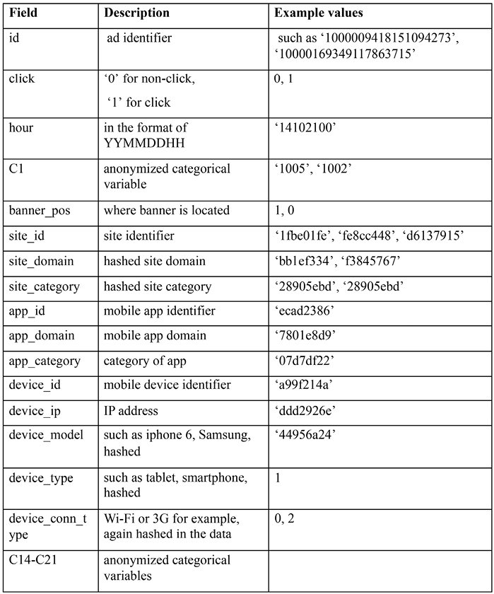
The fields in the raw file are as follows:

Figure 3.12: Description and example values of the dataset

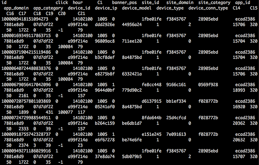
We take a glance at the head of the file by running the following command:

head train | sed 's/,,/, ,/g;s/,,/, ,/g' | column -s, -t

Rather than a simple head train, the output is cleaner as all the columns are aligned:

Figure 3.13: The first few rows of the data

Don’t be scared by the anonymized and hashed values. They are categorical features, and each of their possible values corresponds to a real and meaningful value, but it is presented this way due to the privacy policy. Possibly, C1 means user gender, and 1005 and 1002 represent male and female, respectively.

Now, let’s start by reading the dataset using pandas. That’s right, pandas is extremely good at handling data in a tabular format:

>>> import pandas as pd
>>> n_rows = 300000
>>> df = pd.read_csv("train.csv", nrows=n_rows)

The first 300,000 lines of the file are loaded and stored in a DataFrame. Take a quick look at the first five rows of the DataFrame:

>>> print(df.head(5))
id  click      hour C1 banner_pos   site_id ... C16 C17 C18 C19     C20 C21
0  1.000009e+18      0 14102100 1005          0 1fbe01fe ... 50 1722 0  35 -1 79
1  1.000017e+19      0 14102100 1005          0 1fbe01fe ... 50 1722 0  35 100084 79
2  1.000037e+19      0 14102100 1005          0 1fbe01fe ... 50 1722 0  35 100084 79
3  1.000064e+19      0 14102100 1005          0 1fbe01fe ... 50 1722 0  35 100084 79
4  1.000068e+19      0 14102100 1005          1 fe8cc448 ... 50 2161 0  35 -1 157

The target variable is the click column:

>>> Y = df['click'].values

For the remaining columns, there are several columns that should be removed from the features (id, hour, device_id, and device_ip) as they do not contain much useful information:

>>> X = df.drop(['click', 'id', 'hour', 'device_id', 'device_ip'],
                axis=1).values
>>> print(X.shape)
(300000, 19)

Each sample has 19 predictive attributes.

Next, we need to split the data into training and testing sets. Normally, we do this by randomly picking samples. However, in our case, the samples are in chronological order, as indicated in the hour field. Obviously, we cannot use future samples to predict past ones. Hence, we take the first 90% as training samples and the rest as testing samples:

>>> n_train = int(n_rows * 0.9)
>>> X_train = X[:n_train]
>>> Y_train = Y[:n_train]
>>> X_test = X[n_train:]
>>> Y_test = Y[n_train:]

As mentioned earlier, decision tree models can take in categorical features. However, because the tree-based algorithms in scikit-learn (the current version is 1.4.1 as of early 2024) only allow numeric input, we need to transform the categorical features into numerical ones. But note that, in general, we do not need to do this; for example, the decision tree classifier we developed from scratch earlier can directly take in categorical features.

We will now transform string-based categorical features into one-hot encoded vectors using the OneHotEncoder module from scikit-learn. One-hot encoding was briefly mentioned in Chapter 1, Getting Started with Machine Learning and Python. To recap, it basically converts a categorical feature with k possible values into k binary features. For example, the site category feature with three possible values, news, education, and sports, will be encoded into three binary features, such as is_news, is_education, and is_sports, whose values are either 1 or 0.

We initialize a OneHotEncoder object as follows:

>>> from sklearn.preprocessing import OneHotEncoder
>>> enc = OneHotEncoder(handle_unknown='ignore')

We fit it on the training set as follows:

>>> X_train_enc = enc.fit_transform(X_train)
>>> X_train_enc[0]
<1x8385 sparse matrix of type '<class 'numpy.float64'>'
with 19 stored elements in Compressed Sparse Row format>
>>> print(X_train_enc[0])
  (0, 2)		1.0
  (0, 6)		1.0
  (0, 188)		1.0
  (0, 2608)		1.0
  (0, 2679)		1.0
  (0, 3771)		1.0
  (0, 3885)		1.0
  (0, 3929)		1.0
  (0, 4879)		1.0
  (0, 7315)		1.0
  (0, 7319)		1.0
  (0, 7475)		1.0
  (0, 7824)		1.0
  (0, 7828)		1.0
  (0, 7869)		1.0
  (0, 7977)		1.0
  (0, 7982)		1.0
  (0, 8021)		1.0
  (0, 8189)		1.0

Each converted sample is a sparse vector.

We transform the testing set using the trained one-hot encoder as follows:

>>> X_test_enc = enc.transform(X_test)

Remember, we specified the handle_unknown='ignore' parameter in the one-hot encoder earlier. This is to prevent errors due to any unseen categorical values. To use the previous site category example, if there is a sample with the value movie, all of the three converted binary features (is_news, is_education, and is_sports) become 0. If we do not specify ignore, an error will be raised.

The way we have conducted cross-validation so far is to explicitly split data into folds and repetitively write a for loop to consecutively examine each hyperparameter. To make this less redundant, we’ll introduce a more elegant approach utilizing the GridSearchCV module from scikit-learn. GridSearchCV handles the entire process implicitly, including data splitting, fold generation, cross-training and validation, and finally, an exhaustive search over the best set of parameters. What is left for us is just to specify the hyperparameter(s) to tune and the values to explore for each individual hyperparameter. For demonstration purposes, we will only tweak the max_depth hyperparameter (other hyperparameters, such as min_samples_split and class_weight, are also highly recommended):

>>> from sklearn.tree import DecisionTreeClassifier
>>> parameters = {'max_depth': [3, 10, None]}

We pick three options for the maximal depth – 3, 10, and unbounded. We initialize a decision tree model with Gini Impurity as the metric and 30 as the minimum number of samples required to split further:

>>> decision_tree = DecisionTreeClassifier(criterion='gini',
...                                        min_samples_split=30)

The classification metric should be the AUC of the ROC curve, as it is an imbalanced binary case (only 51,211 out of 300,000 training samples are clicks, which is a 17% positive CTR; I encourage you to figure out the class distribution yourself). As for grid search, we use three-fold (as the training set is relatively small) cross-validation and select the best-performing hyperparameter measured by the AUC:

>>> grid_search = GridSearchCV(decision_tree, parameters,
...                            n_jobs=-1, cv=3, scoring='roc_auc')

Note, n_jobs=-1 means that we use all of the available CPU processors:

>>> grid_search.fit(X_train, y_train)
>>> print(grid_search.best_params_)
{'max_depth': 10}

We use the model with the optimal parameter to predict any future test cases as follows:

>>> decision_tree_best = grid_search.best_estimator_
>>> pos_prob = decision_tree_best.predict_proba(X_test)[:, 1]
>>> from sklearn.metrics import roc_auc_score
>>> print(f'The ROC AUC on testing set is: {roc_auc_score(Y_test,
...           pos_prob):.3f}')
The ROC AUC on testing set is: 0.719

The AUC we can achieve with the optimal decision tree model is 0.72. This does not seem to be very high, but click-through involves many intricate human factors, which is why predicting it is not an easy task. Although we can further optimize the hyperparameters, an AUC of 0.72 is actually pretty good. As a comparison, randomly selecting 17% of the samples to be clicked on will generate an AUC of 0.499:

>>> pos_prob = np.zeros(len(Y_test))
>>> click_index = np.random.choice(len(Y_test),
...                   int(len(Y_test) * 51211.0/300000),
...                   replace=False)
>>> pos_prob[click_index] = 1
>>> print(f'The ROC AUC on testing set using random selection is: {roc_auc_score(Y_test, pos_prob):.3f}')
The ROC AUC on testing set using random selection is: 0.499

Our decision tree model significantly outperforms the random predictor. Looking back, we can see that a decision tree is a sequence of greedy searches for the best splitting point at each step, based on the training dataset. However, this tends to cause overfitting as it is likely that the optimal points only work well for the training samples. Fortunately, ensembling is the technique to correct this, and random forest is an ensemble tree model that usually outperforms a simple decision tree.

Best practice

Here are two best practices for getting data ready for tree-based algorithms:

• Encode categorical features: As mentioned earlier, we need to encode categorical features before feeding them into the models. One-hot encoding and label encoding are popular choices.
• Scale numerical features: We need to pay attention to the scales of numerical features to prevent features with larger scales from dominating the splitting decisions in the tree. Normalization or standardization are commonly used for this purpose.