Implementing neural network-based RL policies for discrete action spaces and decision-making problems
Many environments (both simulated and real) for RL requires the RL agent to choose an action from a list of actions or, in other words, take discrete actions. While simple linear functions can be used to represent policies for such agents, they are often not scalable to complex problems. A non-linear function approximator such as a (deep) neural network can approximate arbitrary functions, even those required to solve complex problems.
The neural network-based policy network is a crucial building block for advanced RL and Deep RL and will be applicable to general, discrete decision-making problems.
By the end of this recipe, you will have an agent with a neural network-based policy implemented in TensorFlow 2.x that can take actions in the Gridworld environment and (with little or no modifications) in any discrete-action space environment.
Getting ready
Activate the tf2rl-cookbook Python virtual environment and run the following to install and import the packages:
pip install --upgrade numpy tensorflow tensorflow_probability seaborn
import seaborn as sns
import tensorflow as tf
from tensorflow import keras
from tensorflow.keras import layers
import tensorflow_probability as tfp
Let's get started.
How to do it…
We will look at policy distribution types that can be used by agents in environments with discrete action spaces:
- Let's begin by creating a binary policy distribution in TensorFlow 2.x using the
tensorflow_probabilitylibrary:binary_policy = tfp.distributions.Bernoulli(probs=0.5) for i in range(5): action = binary_policy.sample(1) print("Action:", action)The preceding code should print something like the following:
Action: tf.Tensor([0], shape=(1,), dtype=int32)
Action: tf.Tensor([1], shape=(1,), dtype=int32)
Action: tf.Tensor([0], shape=(1,), dtype=int32)
Action: tf.Tensor([1], shape=(1,), dtype=int32)
Action: tf.Tensor([1], shape=(1,), dtype=int32)
Important note
The values of the action that you get will differ from what is shown here because they will be sampled from the Bernoulli distribution, which is not a deterministic process.
- Let's quickly visualize the binary policy distribution:
# Sample 500 actions from the binary policy distribution
sample_actions = binary_policy.sample(500)
sns.distplot(sample_actions)
The preceding code will generate a distribution plot as shown here:
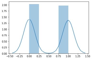
Figure 1.3 – A distribution plot of the binary policy
- In this step, we will be implementing a discrete policy distribution. A categorical distribution over a single discrete variable with k finite categories is referred to as a multinoulli distribution. The generalization of the multinoulli distribution to multiple trials is the multinomial distribution that we will be using to represent discrete policy distributions:
action_dim = 4  # Dimension of the discrete action space
action_probabilities = [0.25, 0.25, 0.25, 0.25]
discrete_policy = tfp.distributions.Multinomial(probs=action_probabilities, total_count=1)
for i in range(5):
    action = discrete_policy.sample(1)
    print(action)
The preceding code should print something along the lines of the following:
Important note
The values of the action that you get will differ from what is shown here because they will be sampled from the multinomial distribution, which is not a deterministic process.
tf.Tensor([[0. 0. 0. 1.]], shape=(1, 4), dtype=float32)
tf.Tensor([[0. 0. 1. 0.]], shape=(1, 4), dtype=float32)
tf.Tensor([[0. 0. 1. 0.]], shape=(1, 4), dtype=float32)
tf.Tensor([[1. 0. 0. 0.]], shape=(1, 4), dtype=float32)
tf.Tensor([[0. 1. 0. 0.]], shape=(1, 4), dtype=float32)
- Next, we visualize the discrete probability distribution:
sns.distplot(discrete_policy.sample(1))
The preceding code will generate a distribution plot, like the one shown here for
discrete_policy: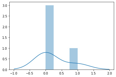
Figure 1.4 – A distribution plot of the discrete policy
- Then, calculate the entropy of a discrete policy:
def entropy(action_probs):
    return -tf.reduce_sum(action_probs * \
                      tf.math.log(action_probs), axis=-1)
action_probabilities = [0.25, 0.25, 0.25, 0.25]
print(entropy(action_probabilities))
- Also, implement a discrete policy class:
class DiscretePolicy(object):
    def __init__(self, num_actions):
        self.action_dim = num_actions
    def sample(self, actino_logits):
        self.distribution = tfp.distributions.Multinomial(logits=action_logits, total_count=1)
        return self.distribution.sample(1)
    def get_action(self, action_logits):
        action = self.sample(action_logits)
        return np.where(action)[-1]
        # Return the action index
    def entropy(self, action_probabilities):
        return – tf.reduce_sum(action_probabilities * tf.math.log(action_probabilities), axis=-1)
- Now we implement a helper method to evaluate the agent in a given environment:
def evaluate(agent, env, render=True):
    obs, episode_reward, done, step_num = env.reset(),
                                          0.0, False, 0
    while not done:
        action = agent.get_action(obs)
        obs, reward, done, info = env.step(action)
        episode_reward += reward
        step_num += 1
        if render:
            env.render()
    return step_num, episode_reward, done, info
- Let's now implement a neural network Brain class using TensorFlow 2.x:
class Brain(keras.Model):
    def __init__(self, action_dim=5,
                 input_shape=(1, 8 * 8)):
        """Initialize the Agent's Brain model
        Args:
            action_dim (int): Number of actions
        """
        super(Brain, self).__init__()
        self.dense1 = layers.Dense(32, input_shape=\
                          input_shape, activation="relu")
        self.logits = layers.Dense(action_dim)
    def call(self, inputs):
        x = tf.convert_to_tensor(inputs)
        if len(x.shape) >= 2 and x.shape[0] != 1:
            x = tf.reshape(x, (1, -1))
        return self.logits(self.dense1(x))
    def process(self, observations):
# Process batch observations using `call(inputs)` behind-the-scenes
        action_logits = \
                     self.predict_on_batch(observations)
        return action_logits
- Let's now implement a simple agent class that uses a
DiscretePolicyobject to act in discrete environments:class Agent(object): def __init__(self, action_dim=5, input_dim=(1, 8 * 8)): self.brain = Brain(action_dim, input_dim) self.policy = DiscretePolicy(action_dim) def get_action(self, obs): action_logits = self.brain.process(obs) action = self.policy.get_action( np.squeeze(action_logits, 0)) return action
- Let's now test the agent in
GridworldEnv:from envs.gridworld import GridworldEnv env = GridworldEnv() agent = Agent(env.action_space.n, env.observation_space.shape) steps, reward, done, info = evaluate(agent, env) print(f"steps:{steps} reward:{reward} done:{done} info:{info}") env.close()
This shows how to implement the policy. We will see how this works in the following section.
How it works…
One of the central components of an RL agent is the policy function that maps between observations and actions. Formally, a policy is a distribution over actions that prescribes the probabilities of choosing an action given an observation.
In environments where the agent can take at most two different actions, for example, in a binary action space, we can represent the policy using a Bernoulli distribution, where the probability of taking action 0 is given by 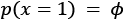 , and the probability of taking action 1 is given by
 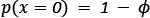 , which gives rise to the following probability distribution:

A discrete probability distribution can be used to represent an RL agent's policy when the agent can take one of k possible actions in an environment.
In a general sense, such distributions can be used to describe the possible results of a random variable that can take one of k possible categories and is therefore also called a categorical distribution. This is a generalization of the Bernoulli distribution to k-way events and is therefore a multinoulli distribution.