Running a pretrained VGG model
We have already discussed LeNet and AlexNet, two of the foundational CNN architectures. As we progress in the chapter, we will explore increasingly complex CNN models. That being said, the key principles in building these model architectures will be the same. We will see a modular model-building approach in putting together convolutional layers, pooling layers, and fully connected layers into blocks/modules and then stacking these blocks sequentially or in a branched manner. In this section, we look at the successor to AlexNet – VGGNet.
The name VGG is derived from the Visual Geometry Group of Oxford University, where this model was invented. Compared to the 8 layers and 60 million parameters of AlexNet, VGG consists of 13 layers (10 convolutional layers and 3 fully connected layers) and 138 million parameters. VGG basically stacks more layers onto the AlexNet architecture with smaller convolution kernels (2x2 or 3x3).
Hence, VGG’s novelty lies in the unprecedented level of depth that it brings with its architecture. Figure 2.12 shows the VGG architecture:

Figure 2.12: VGG16 architecture
The preceding VGG architecture is called VGG13, because of the 13 layers. Other variants are VGG16 and VGG19, consisting of 16 and 19 layers, respectively. There is another set of variants – VGG13_bn, VGG16_bn, and VGG19_bn, where bn suggests that these models also consist of batch-normalization layers.
PyTorch’s torchvision.model sub-package provides the pretrained VGG model (with all of the six variants discussed earlier) trained on the ImageNet dataset. In the following exercise, we will use the pretrained VGG13 model to make predictions on a small dataset of bees and ants (used in the previous exercise). We will focus on the key pieces of code here, as most other parts of our code will overlap with that of the previous exercises. We can always refer to our notebooks to explore the full code [7]:
- First, we need to import dependencies, including
torchvision.models. - Download the data and set up the ants and bees dataset and dataloader, along with the transformations.
- In order to make predictions on these images, we will need to download the 1,000 labels of the ImageNet dataset [8].
- Once downloaded, we need to create a mapping between the class indices 0 to 999 and the corresponding class labels, as shown here:
import ast
with open('./imagenet1000_clsidx_to_labels.txt') as f:
    classes_data = f.read()
classes_dict = ast.literal_eval(classes_data)
print({k: classes_dict[k] for k in list(classes_dict)[:5]})
This should output the first five class mappings, as shown below:
{0: 'tench, Tinca tinca', 1: 'goldfish, Carassius auratus', 2: 'great white shark, white shark, man-eater, man-eating shark, Carcharodon carcharias', 3: 'tiger shark, Galeocerdo cuvieri', 4: 'hammerhead, hammerhead shark'}
- Define the model prediction visualization function that takes in the pretrained model object and the number of images to run predictions on. This function should output the images with predictions.
- Load the pretrained
VGG13model:model_finetune = models.vgg13(pretrained=True)
The VGG13 model is downloaded in this step.
FAQ – What is the disk size of a VGG13 model?
A VGG13 model will consume roughly 508 MB on your hard disk.
- Finally, we run predictions on our ants and bees dataset using this pretrained model:
visualize_predictions(model_finetune)
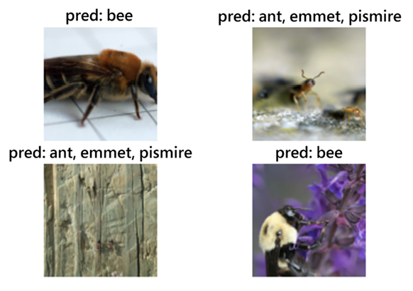
This should output the following:

Figure 2.13: VGG13 predictions
The VGG13 model trained on an entirely different dataset seems to predict all the test samples correctly in the ants and bees dataset. Basically, the model grabs the two most similar animals from the dataset out of the 1,000 classes and finds them in the images. By doing this exercise, we see that the model is still able to extract relevant visual features out of the images and the exercise demonstrates the utility of PyTorch’s out-of-the-box inference feature.
In the next section, we are going to study a different type of CNN architecture – one that involves modules that have multiple parallel convolutional layers. The modules are called Inception modules and the resulting network is called the Inception Network – named after the movie Inception – because this model contains several branching modules much like the branching dreams of the movie. We will explore the various parts of this network and the reasoning behind its success. We will also build the Inception modules and the Inception network architecture using PyTorch.


