Search icon CANCEL
Arrow left icon
Explore Products
Best Sellers
New Releases
Books
Videos
Audiobooks
Learning Hub
Conferences
Free Learning
Arrow right icon
Data Science  with Python

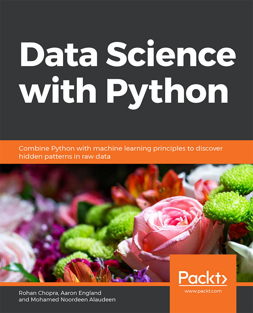
Data Science with Python: Combine Python with machine learning principles to discover hidden patterns in raw data

Arrow left icon
Profile Icon Rohan Chopra Profile Icon England Profile Icon Mohamed Noordeen Alaudeen
Arrow right icon
€15.99 €23.99
Full star icon Full star icon Full star icon Empty star icon Empty star icon 3 (1 Ratings)
eBook Jul 2019 426 pages 1st Edition
eBook
€15.99 €23.99
Paperback
€29.99
Subscription
Free Trial
Renews at €18.99p/m
eBook
€15.99 €23.99
Paperback
€29.99
Subscription
Free Trial
Renews at €18.99p/m

What do you get with eBook?

Product feature icon Instant access to your Digital eBook purchase
Product feature icon Download this book in EPUB and PDF formats
Product feature icon Access this title in our online reader with advanced features
Product feature icon DRM FREE - Read whenever, wherever and however you want
Product feature icon AI Assistant (beta) to help accelerate your learning
Table of content icon View table of contents Preview book icon Preview Book

Data Science with Python

Introduction to Data Science and Data Pre-Processing

Learning Objectives

By the end of this chapter, you will be able to:

  • Use various Python machine learning libraries
  • Handle missing data and deal with outliers
  • Perform data integration to bring together data from different sources
  • Perform data transformation to convert data into a machine-readable form
  • Scale data to avoid problems with values of different magnitudes
  • Split data into train and test datasets
  • Describe the different types of machine learning
  • Describe the different performance measures of a machine learning model

This chapter introduces data science and covers the various processes included in the building of machine learning models, with a particular focus on pre-processing.

Python Libraries

Throughout this book, we'll be using various Python libraries, including pandas, Matplotlib, Seaborn, and scikit-learn.

pandas

pandas is an open source package that has many functions for loading and processing data in order to prepare it for machine learning tasks. It also has tools that can be used to analyze and manipulate data. Data can be read from many formats using pandas. We will mainly be using CSV data throughout this book. To read CSV data, you can use the read_csv() function by passing filename.csv as an argument. An example of this is shown here:

>>> import pandas as pd

>>> pd.read_csv("data.csv")

In the preceding code, pd is an alias name given to pandas. It is not mandatory to give an alias. To visualize a pandas DataFrame, you can use the head() function to list the top five rows. This will be demonstrated in one of the following exercises.

Note

Please visit the following link to learn more about pandas: https://pandas.pydata.org/pandas-docs/stable/.

NumPy

NumPy is one of the main packages that Python has to offer. It is mainly used in practices related to scientific computing and when working on mathematical operations. It comprises of tools that enable us to work with arrays and array objects.

Matplotlib

Matplotlib is a data visualization package. It is useful for plotting data points in a 2D space with the help of NumPy.

Seaborn

Seaborn is also a data visualization library that is based on matplotlib. Visualizations created using Seaborn are far more attractive than ones created using matplotlib in terms of graphics.

scikit-learn

scikit-learn is a Python package used for machine learning. It is designed in such a way that it interoperates with other numeric and scientific libraries in Python to achieve the implementation of algorithms.

These ready-to-use libraries have gained interest and attention from developers, especially in the data science space. Now that we have covered the various libraries in Python, in the next section we'll explore the roadmap for building machine learning models.

Roadmap for Building Machine Learning Models

The roadmap for building machine learning models is straightforward and consists of five major steps, which are explained here:

  • Data Pre-processing

    This is the first step in building a machine learning model. Data pre-processing refers to the transformation of data before feeding it into the model. It deals with the techniques that are used to convert unusable raw data into clean reliable data.

    Since data collection is often not performed in a controlled manner, raw data often contains outliers (for example, age = 120), nonsensical data combinations (for example, model: bicycle, type: 4-wheeler), missing values, scale problems, and so on. Because of this, raw data cannot be fed into a machine learning model because it might compromise the quality of the results. As such, this is the most important step in the process of data science.

  • Model Learning

    After pre-processing the data and splitting it into train/test sets (more on this later), we move on to modeling. Models are nothing but sets of well-defined methods called algorithms that use pre-processed data to learn patterns, which can later be used to make predictions. There are different types of learning algorithms, including supervised, semi-supervised, unsupervised, and reinforcement learning. These will be discussed later.

  • Model Evaluation

    In this stage, the models are evaluated with the help of specific performance metrics. With these metrics, we can go on to tune the hyperparameters of a model in order to improve it. This process is called hyperparameter optimization. We will repeat this step until we are satisfied with the performance.

  • Prediction

    Once we are happy with the results from the evaluation step, we will then move on to predictions. Predictions are made by the trained model when it is exposed to a new dataset. In a business setting, these predictions can be shared with decision makers to make effective business choices.

  • Model Deployment

    The whole process of machine learning does not just stop with model building and prediction. It also involves making use of the model to build an application with the new data. Depending on the business requirements, the deployment may be a report, or it may be some repetitive data science steps that are to be executed. After deployment, a model needs proper management and maintenance at regular intervals to keep it up and running.

This chapter will mainly focus on pre-processing. We will cover the different tasks involved in data pre-processing, such as data representation, data cleaning, and others.

Data Representation

The main objective of machine learning is to build models that understand data and find underlying patterns. In order to do so, it is very important to feed the data in a way that is interpretable by the computer. To feed the data into a model, it must be represented as a table or a matrix of the required dimensions. Converting your data into the correct tabular form is one of the first steps before pre-processing can properly begin.

Data Represented in a Table

Data should be arranged in a two-dimensional space made up of rows and columns. This type of data structure makes it easy to understand the data and pinpoint any problems. An example of some raw data stored as a CSV (comma separated values) file is shown here:

Figure 1.1: Raw data in CSV format

The representation of the same data in a table is as follows:

Figure 1.2: CSV data in table format

If you compare the data in CSV and table formats, you will see that there are missing values in both. We will cover what to do with these later in the chapter. To load a CSV file and work on it as a table, we use the pandas library. The data here is loaded into tables called DataFrames.

Note

To learn more about pandas, visit the following link: http://pandas.pydata.org/pandas-docs/version/0.15/tutorials.html.

Independent and Target Variables

The DataFrame that we use contains variables or features that can be classified into two categories. These are independent variables (also called predictor variables) and dependent variables (also called target variables). Independent variables are used to predict the target variable. As the name suggests, independent variables should be independent of each other. If they are not, this will need to be addressed in the pre-processing (cleaning) stage.

Independent Variables

These are all the features in the DataFrame except the target variable. They are of size (m, n), where m is the number of observations and n is the number of features. These variables must be normally distributed and should NOT contain:

  • Missing or NULL values
  • Highly categorical data features or high cardinality (these terms will be covered in more detail later)
  • Outliers
  • Data on different scales
  • Human error
  • Multicollinearity (independent variables that are correlated)
  • Very large independent feature sets (too many independent variables to be manageable)
  • Sparse data
  • Special characters

Feature Matrix and Target Vector

A single piece of data is called a scalar. A group of scalars is called a vector, and a group of vectors is called a matrix. A matrix is represented in rows and columns. Feature matrix data is made up of independent columns, and the target vector depends on the feature matrix columns. To get a better understanding of this, let's look at the following table:

Figure 1.3: Table containing car details

As you can see in the table, there are various columns: Car Model, Car Capacity, Car Brand, and Car Price. All columns except Car Price are independent variables and represent the feature matrix. Car Price is the dependent variable that depends on the other columns (Car Model, Car Capacity, and Car Brand). It is a target vector because it depends on the feature matrix data. In the next section, we'll go through an exercise based on features and a target matrix to get a thorough understanding.

Note 

All exercises and activities will be primarily developed in Jupyter Notebook. It is recommended to keep a separate notebook for different assignments unless advised not to. Also, to load a sample dataset, the pandas library will be used, because it displays the data as a table. Other ways to load data will be explained in further sections.

Exercise 1: Loading a Sample Dataset and Creating the Feature Matrix and Target Matrix

In this exercise, we will be loading the House_price_prediction dataset into the pandas DataFrame and creating feature and target matrices. The House_price_prediction dataset is taken from the UCI Machine Learning Repository. The data was collected from various suburbs of the USA and consists of 5,000 entries and 6 features related to houses. Follow these steps to complete this exercise:

Note

The House_price_prediction dataset can be found at this location: https://github.com/TrainingByPackt/Data-Science-with-Python/blob/master/Chapter01/Data/USA_Housing.csv.

  1. Open a Jupyter notebook and add the following code to import pandas:

    import pandas as pd

  2. Now we need to load the dataset into a pandas DataFrame. As the dataset is a CSV file, we'll be using the read_csv() function to read the data. Add the following code to do this:

    dataset = "https://github.com/TrainingByPackt/Data-Science-with-Python/blob/master/Chapter01/Data/USA_Housing.csv"

    df = pd.read_csv(dataset, header = 0)

    As you can see in the preceding code, the data is stored in a variable named df.

  3. To print all the column names of the DataFrame, we'll use the df.columns command. Write the following code in the notebook:

    df.columns

    The preceding code generates the following output:

    Figure 1.4: List of columns present in the dataframe
    Figure 1.4: List of columns present in the dataframe
  4. The dataset contains n number of data points. We can find the total number of rows using the following command:

    df.index

    The preceding code generates the following output:

    Figure 1.5: Total Index in the dataframe
    Figure 1.5: Total Index in the dataframe

    As you can see in the preceding figure, our dataset contains 5000 rows, from index 0 to 5000.

    Note

    You can use the set_index() function in pandas to convert a column into an index of rows in a DataFrame. This is a bit like using the values in that column as your row labels.

    Dataframe.set_index('column name', inplace = True')'

  5. Let's set the Address column as an index and reset it back to the original DataFrame. The pandas library provides the set_index() method to convert a column into an index of rows in a DataFrame. Add the following code to implement this:

    df.set_index('Address', inplace=True)

    df

    The preceding code generates the following output:

    Figure 1.6: DataFrame with an indexed Address column
    Figure 1.6: DataFrame with an indexed Address column

    The inplace parameter in the set_index() function is by default set to False. If the value is changed to True, then whatever operation we perform the content of the DataFrame changes directly without the copy being created.

  6. In order to reset the index of the given object, we use the reset_index() function. Write the following code to implement this:

    df.reset_index(inplace=True)

    df

    The preceding code generates the following output:

    Figure 1.7: DataFrame with the index reset
    Figure 1.7: DataFrame with the index reset

    Note

    The index is like a name given to a row and column. Rows and columns both have an index. You can index by row/column number or row/column name.

  7. We can retrieve the first four rows and the first three columns using a row number and column number. This can be done using the iloc indexer in pandas, which retrieves data using index positions. Add the following code to do this:

    df.iloc[0:4 , 0:3]

    Figure 1.8: Dataset of four rows and three columns
    Figure 1.8: Dataset of four rows and three columns
  8. To retrieve the data using labels, we use the loc indexer. Add the following code to retrieve the first five rows of the Income and Age columns:

    df.loc[0:4 , ["Avg. Area Income", "Avg. Area House Age"]]

    Figure 1.9: Dataset of five rows and two columns
    Figure 1.9: Dataset of five rows and two columns
  9. Now create a variable called X to store the independent features. In our dataset, we will consider all features except Price as independent variables, and we will use the drop() function to include them. Once this is done, we print out the top five instances of the X variable. Add the following code to do this:

    X = df.drop('Price', axis=1)

    X.head()

    The preceding code generates the following output:

    Figure 1.10: Dataset showing the first five rows of the feature matrix
    Figure 1.10: Dataset showing the first five rows of the feature matrix

    Note

    The default number of instances that will be taken for the head is five, so if you don't specify the number then it will by default output five observations. The axis parameter in the preceding screenshot denotes whether you want to drop the label from rows (axis = 0) or columns (axis = 1).

  10. Print the shape of your newly created feature matrix using the X.shape command. Add the following code to do this:

    X.shape

    The preceding code generates the following output:

    Figure 1.11: Shape of the feature matrix

    In the preceding figure, the first value indicates the number of observations in the dataset (5000), and the second value represents the number of features (6).

  11. Similarly, we will create a variable called y that will store the target values. We will use indexing to grab the target column. Indexing allows you to access a section of a larger element. In this case, we want to grab the column named Price from the df DataFrame. Then, we want to print out the top 10 values of the variable. Add the following code to implement this:

    y = df['Price']

    y.head(10)

    The preceding code generates the following output:

    Figure 1.12: Dataset showing the first 10 rows of the target matrix
    Figure 1.12: Dataset showing the first 10 rows of the target matrix
  12. Print the shape of your new variable using the y.shape command. The shape should be one-dimensional, with a length equal to the number of observations (5000) only. Add the following code to implement this:

    y.shape

    The preceding code generates the following output:

Figure 1.13: Shape of the target matrix

You have successfully created the feature and target matrices of a dataset. You have completed the first step in the process of building a predictive model. This model will learn the patterns from the feature matrix (columns in X) and how they map to the values in the target vector (y). These patterns can then be used to predict house prices from new data based on the features of those new houses.

In the next section, we will explore more steps involved in pre-processing.

Data Cleaning

Data cleaning includes processes such as filling in missing values and handling inconsistencies. It detects corrupt data and replaces or modifies it.

Missing Values

The concept of missing values is important to understand if you want to master the skill of successful management and understanding of data. Let's take a look at the following figure:

Figure 1.14: Bank customer credit data

As you can see, the data belongs to a bank; each row is a separate customer and each column contains their details, such as age and credit amount. There are some cells that have either NA or are just empty. This is missing data. Each piece of information about the customer is crucial for the bank. If any of the information is missing, then it will be difficult for the bank to predict the risk of providing a loan to the customer.

Handling Missing Data

Intelligent handling of missing data will result in building a robust model capable of handling complex tasks. There are many ways to handle missing data. Let's now look at some of those ways.

Removing the Data

Checking missing values is the first and the most important step in data pre-processing. A model cannot accept data with missing values. This is a very simple and commonly used method to handle missing values: we delete a row if the missing value corresponds to the places in the row, or we delete a column if it has more than 70%-75% of missing data. Again, the threshold value is not fixed and depends on how much you wish to fix.

The benefit of this approach is that it is quick and easy to do, and in many cases no data is better than bad data. The drawback is that you may end up losing important information, because you're deleting a whole feature based on a few missing values.

Exercise 2: Removing Missing Data

In this exercise, we will be loading the Banking_Marketing.csv dataset into the pandas DataFrame and handling the missing data. This dataset is related to direct marketing campaigns of a Portuguese banking institution. The marketing campaigns involved phone calls to clients to try and get them to subscribe to a particular product. The dataset contains the details of each client contacted, and whether they subscribed to the product. Follow these steps to complete this exercise:

Note

The Banking_Marketing.csv dataset can be found at this location: https://github.com/TrainingByPackt/Data-Science-with-Python/blob/master/Chapter01/Data/Banking_Marketing.csv.

  1. Open a Jupyter notebook. Insert a new cell and add the following code to import pandas and fetch the Banking_Marketing.csv dataset:

    import pandas as pd

    dataset = 'https://github.com/TrainingByPackt/Data-Science-with-Python/blob/master/Chapter01/Data/Banking_Marketing.csv'

    #reading the data into the dataframe into the object data

    df = pd.read_csv(dataset, header=0)

  2. Once you have fetched the dataset, print the datatype of each column. To do so, use the dtypes attribute from the pandas DataFrame:

    df.dtypes

    The preceding code generates the following output:

    Figure 1.15: Data types of each feature
    Figure 1.15: Data types of each feature
  3. Now we need to find the missing values for each column. In order to do that, we use the isna() function provided by pandas:

    df.isna().sum()

    The preceding code generates the following output:

    Figure 1.16: Missing values of each column in the dataset
    Figure 1.16: Missing values of each column in the dataset

    In the preceding figure, we can see that there is data missing from three columns, namely age, contact, and duration. There are two NAs in the age column, six NAs in contact, and seven NAs in duration.

  4. Once you have figured out all the missing details, we remove all the missing rows from the DataFrame. To do so, we use the dropna() function:

    #removing Null values

    data = data.dropna()

  5. To check whether the missing vales are still present, use the isna() function:

    df.isna().sum()

    The preceding code generates the following output:

Figure 1.17: Each column of the dataset with zero missing values

You have successfully removed all missing data from the DataFrame. In the next section, we'll look at the second method of dealing with missing data, which uses imputation.

Mean/Median/Mode Imputation

In the case of numerical data, we can compute its mean or median and use the result to replace missing values. In the case of the categorical (non-numerical) data, we can compute its mode to replace the missing value. This is known as imputation.

The benefit of using imputation, rather than just removing data, is that it prevents data loss. The drawback is that you don't know how accurate using the mean, median, or mode is going to be in a given situation.

Let's look at an exercise in which we will use imputation method to solve missing data problems.

Exercise 3: Imputing Missing Data

In this exercise, we will be loading the Banking_Marketing.csv dataset into the pandas DataFrame and handle the missing data. We'll make use of the imputation method. Follow these steps to complete this exercise:

Note

The Banking_Marketing.csv dataset can be found at this location: https://github.com/TrainingByPackt/Data-Science-with-Python/blob/master/Chapter01/Data/Banking_Marketing.csv.

  1. Open a Jupyter notebook and add a new cell. Load the dataset into the pandas DataFrame. Add the following code to do this:

    import pandas as pd

    dataset = 'https://github.com/TrainingByPackt/Data-Science-with-Python/blob/master/Chapter01/Data/Banking_Marketing.csv'

    df = pd.read_csv(dataset, header=0)

  2. Impute the numerical data of the age column with its mean. To do so, first find the mean of the age column using the mean() function of pandas, and then print it:

    mean_age = df.age.mean()

    print(mean_age)

    The preceding code generates the following output:

    Figure 1.18: Mean of the age column
    Figure 1.18: Mean of the age column
  3. Once this is done, impute the missing data with its mean using the fillna() function. This can be done with the following code:

    df.age.fillna(mean_age, inplace=True)

  4. Now we impute the numerical data of the duration column with its median. To do so, first find the median of the duration column using the median() function of the pandas. Add the following code to do so:

    median_duration = df.duration.median()

    print(median_duration)

    Figure 1.19: Median of the duration
    Figure 1.19: Median of the duration
  5. Impute the missing data of the duration with its median using the fillna() function.

    df. duration.fillna(median_duration,inplace=True)

  6. Impute the categorical data of the contact column with its mode. To do so, first, find the mode of the contact column using the mode() function of pandas. Add the following code to do this:

    mode_contact = df.contact.mode()[0]

    print(mode_contact)

    Figure 1.20: Mode of the contact
  7. Impute the missing data of the contact column with its mode using the fillna() function. Add the following code to do this:

    df.contact.fillna(mode_contact,inplace=True)

    Unlike mean and median, there may be more than one mode in a column. So, we just take the first mode with index 0.

You have successfully imputed the missing data in different ways and made the data complete and clean.

Another part of data cleaning is dealing with outliers, which will be discussed in the next section.

Outliers

Outliers are values that are very large or very small with respect to the distribution of the other data. We can only find outliers in numerical data. Box plots are one good way to find the outliers in a dataset, as you can see in the following figure:

Figure 1.21: Sample of outliers in a box plot

Note

An outlier is not always bad data! With the help of business understanding and client interaction, you can discern whether to remove or retain the outlier.

Let's learn how to find outliers using a simple example. Consider a sample dataset of temperatures from a place at different times:

71, 70, 90, 70, 70, 60, 70, 72, 72, 320, 71, 69

We can now do the following:

  1. First, we'll sort the data:

    60,69, 70, 70, 70, 70, 71, 71, 72, 72, 90, 320

  2. Next, we'll calculate the median (Q2). The median is the middle data after sorting.

    Here, the middle terms are 70 and 71 after sorting the list.

    The median is (70 + 71) / 2 = 70.5

  3. Then we'll calculate the lower quartile (Q1). Q1 is the middle value (median) of the first half of the dataset.

    First half of the data = 60, 69, 70, 70, 70, 70

    Points 3 and 4 of the bottom 6 are both equal to 70.

    The average is (70 + 70) / 2 = 70

    Q1 = 70

  4. Then we calculate the upper quartile (Q3).

    Q3 is the middle value (median) of the second half of the dataset.

    Second half of the data = 71, 71, 72, 72, 90, 320

    Points 3 and 4 of the upper 6 are 72 and 72.

    The average is (72 + 72) / 2 = 72

    Q3 = 72

  5. Then we find the interquartile range (IQR).

    IQR = Q3 – Q1 = 72 – 70

    IQR = 2

  6. Next, we find the upper and lower fences.

    Lower fence = Q1 – 1.5 (IQR) = 70 – 1.5(2) = 67

    Upper fence = Q3 + 1.5 (IQR) = 71.5 + 1.5(2) = 74.5

    Boundaries of our fences = 67 and 74.5

Any data points lower than the lower fence and greater than the upper fence are outliers. Thus, the outliers from our example are 60, 90 and 320.

Exercise 4: Finding and Removing Outliers in Data

In this exercise, we will be loading the german_credit_data.csv dataset into the pandas DataFrame and removing the outliers. The dataset contains 1,000 entries with 20 categorial/symbolic attributes prepared by Prof. Hofmann. In this dataset, each entry represents a person who takes credit from a bank. Each person is classified as a good or bad credit risk according to the set of attributes. Follow these steps to complete this exercise:

Note

The link to the german_credit_data.csv dataset can be found here: https://github.com/TrainingByPackt/Data-Science-with-Python/blob/master/Chapter01/Data/german_credit_data.csv.

  1. Open a Jupyter notebook and add a new cell. Write the following code to import the necessary libraries: pandas, NumPy, matplotlib, and seaborn. Fetch the dataset and load it into the pandas DataFrame. Add the following code to do this:

    import pandas as pd

    import numpy as np

    %matplotlib inline

    import seaborn as sbn

    dataset = 'https://github.com/TrainingByPackt/Data-Science-with-Python/blob/master/Chapter01/Data/german_credit_data.csv'

    #reading the data into the dataframe into the object data

    df = pd.read_csv(dataset, header=0)

    In the preceding code, %matplotlib inline is a magic function that is essential if we want the plot to be visible in the notebook.

  2. This dataset contains an Age column. Let's plot a boxplot of the Age column. To do so, use the boxplot() function from the seaborn library:

    sbn.boxplot(df['Age'])

    The preceding code generates the following output:

    Figure 1.22: A box plot of the Age column
    Figure 1.22: A box plot of the Age column

    We can see that some data points are outliers in the boxplot.

  3. The boxplot uses the IQR method to display the data and the outliers (the shape of the data). But in order to print an outlier, we use a mathematical formula to retrieve it. Add the following code to find the outliers of the Age column using the IQR method:

    Q1 = df["Age"].quantile(0.25)

    Q3 = df["Age"].quantile(0.75)

    IQR = Q3 - Q1

    print(IQR)

    >>> 15.0

    In the preceding code, Q1 is the first quartile and Q3 is the third quartile.

  4. Now we find the upper fence and lower fence by adding the following code, and print all the data above the upper fence and below the lower fence. Add the following code to do this:

    Lower_Fence = Q1 - (1.5 * IQR)

    Upper_Fence = Q3 + (1.5 * IQR)

    print(Lower_Fence)

    print(Upper_Fence)

    >>> 4.5

    >>> 64.5

  5. To print all the data above the upper fence and below the lower fence, add the following code:

    df[((df["Age"] < Lower_Fence) |(df["Age"] > Upper_Fence))]

    The preceding code generates the following output:

    Figure 1.23: Outlier data based on the Age column
    Figure 1.23: Outlier data based on the Age column
  6. Filter out the outlier data and print only the potential data. To do so, just negate the preceding result using the ~ operator:

    df = df[~((df ["Age"] < Lower_Fence) |(df["Age"] > Upper_Fence))]

    df

    The preceding code generates the following output:

Figure 1.24: Potential data based on the Age column

You have successfully found the outliers using the IQR. In the next section, we will explore another method of pre-processing called data integration.

Data Integration

So far, we've made sure to remove the impurities in data and make it clean. Now, the next step is to combine data from different sources to get a unified structure with more meaningful and valuable information. This is mostly used if the data is segregated into different sources. To make it simple, let's assume we have data in CSV format in different places, all talking about the same scenario. Say we have some data about an employee in a database. We can't expect all the data about the employee to reside in the same table. It's possible that the employee's personal data will be located in one table, the employee's project history will be in a second table, the employee's time-in and time-out details will be in another table, and so on. So, if we want to do some analysis about the employee, we need to get all the employee data in one common place. This process of bringing data together in one place is called data integration. To do data integration, we can merge multiple pandas DataFrames using the merge function.

Let's solve an exercise based on data integration to get a clear understanding of it.

Exercise 5: Integrating Data

In this exercise, we'll merge the details of students from two datasets, namely student.csv and marks.csv. The student dataset contains columns such as Age, Gender, Grade, and Employed. The marks.csv dataset contains columns such as Mark and City. The Student_id column is common between the two datasets. Follow these steps to complete this exercise:

Note

The student.csv dataset can be found at this location: https://github.com/TrainingByPackt/Data-Science-with-Python/blob/master/Chapter01/Data/student.csv.

The marks.csv dataset can be found at this location: https://github.com/TrainingByPackt/Data-Science-with-Python/blob/master/Chapter01/Data/mark.csv.

  1. Open a Jupyter notebook and add a new cell. Write the following code to import pandas and load the student.csv and marks.csv datasets into the df1 and df2 pandas DataFrames:

    import pandas as pd

    dataset1 = "https://github.com/TrainingByPackt/Data-Science-with-Python/blob/master/Chapter01/Data/student.csv"

    dataset2 = "https://github.com/TrainingByPackt/Data-Science-with-Python/blob/master/Chapter01/Data/mark.csv"

    df1 = pd.read_csv(dataset1, header = 0)

    df2 = pd.read_csv(dataset2, header = 0)

  2. To print the first five rows of the first DataFrame, add the following code:

    df1.head()

    The preceding code generates the following output:

    Figure 1.25: The first five rows of the first DataFrame
    Figure 1.25: The first five rows of the first DataFrame
  3. To print the first five rows of the second DataFrame, add the following code:

    df2.head()

    The preceding code generates the following output:

    Figure 1.26: The first five rows of the second DataFrame
    Figure 1.26: The first five rows of the second DataFrame
  4. Student_id is common to both datasets. Perform data integration on both the DataFrames with respect to the Student_id column using the pd.merge() function, and then print the first 10 values of the new DataFrame:

    df = pd.merge(df1, df2, on = 'Student_id')

    df.head(10)

Figure 1.27: First 10 rows of the merged DataFrame

Here, the data of the df1 DataFrame is merged with the data of the df2 DataFrame. The merged data is stored inside a new DataFrame called df.

We have now learned how to perform data integration. In the next section, we'll explore another pre-processing task, data transformation.

Data Transformation

Previously, we saw how we can combine data from different sources into a unified dataframe. Now, we have a lot of columns that have different types of data. Our goal is to transform the data into a machine-learning-digestible format. All machine learning algorithms are based on mathematics. So, we need to convert all the columns into numerical format. Before that, let's see all the different types of data we have.

Taking a broader perspective, data is classified into numerical and categorical data:

  • Numerical: As the name suggests, this is numeric data that is quantifiable.
  • Categorical: The data is a string or non-numeric data that is qualitative in nature.

Numerical data is further divided into the following:

  • Discrete: To explain in simple terms, any numerical data that is countable is called discrete, for example, the number of people in a family or the number of students in a class. Discrete data can only take certain values (such as 1, 2, 3, 4, etc).
  • Continuous: Any numerical data that is measurable is called continuous, for example, the height of a person or the time taken to reach a destination. Continuous data can take virtually any value (for example, 1.25, 3.8888, and 77.1276).

Categorical data is further divided into the following:

  • Ordered: Any categorical data that has some order associated with it is called ordered categorical data, for example, movie ratings (excellent, good, bad, worst) and feedback (happy, not bad, bad). You can think of ordered data as being something you could mark on a scale.
  • Nominal: Any categorical data that has no order is called nominal categorical data. Examples include gender and country.

From these different types of data, we will focus on categorical data. In the next section, we'll discuss how to handle categorical data.

Handling Categorical Data

There are some algorithms that can work well with categorical data, such as decision trees. But most machine learning algorithms cannot operate directly with categorical data. These algorithms require the input and output both to be in numerical form. If the output to be predicted is categorical, then after prediction we convert them back to categorical data from numerical data. Let's discuss some key challenges that we face while dealing with categorical data:

  • High cardinality: Cardinality means uniqueness in data. The data column, in this case, will have a lot of different values. A good example is User ID – in a table of 500 different users, the User ID column would have 500 unique values.
  • Rare occurrences: These data columns might have variables that occur very rarely and therefore would not be significant enough to have an impact on the model.
  • Frequent occurrences: There might be a category in the data columns that occurs many times with very low variance, which would fail to make an impact on the model.
  • Won't fit: This categorical data, left unprocessed, won't fit our model.

Encoding

To address the problems associated with categorical data, we can use encoding. This is the process by which we convert a categorical variable into a numerical form. Here, we will look at three simple methods of encoding categorical data.

Replacing

This is a technique in which we replace the categorical data with a number. This is a simple replacement and does not involve much logical processing. Let's look at an exercise to get a better idea of this.

Exercise 6: Simple Replacement of Categorical Data with a Number

In this exercise, we will use the student dataset that we saw earlier. We will load the data into a pandas dataframe and simply replace all the categorical data with numbers. Follow these steps to complete this exercise:

Note

The student dataset can be found at this location: https://github.com/TrainingByPackt/Data-Science-with-Python/blob/master/Chapter01/Data/student.csv.

  1. Open a Jupyter notebook and add a new cell. Write the following code to import pandas and then load the dataset into the pandas dataframe:

    import pandas as pd

    import numpy as np

    dataset = "https://github.com/TrainingByPackt/Data-Science-with-Python/blob/master/Chapter01/Data/student.csv"

    df = pd.read_csv(dataset, header = 0)

  2. Find the categorical column and separate it out with a different dataframe. To do so, use the select_dtypes() function from pandas:

    df_categorical = df.select_dtypes(exclude=[np.number])

    df_categorical

    The preceding code generates the following output:

    Figure 1.28: Categorical columns of the dataframe
    Figure 1.28: Categorical columns of the dataframe
  3. Find the distinct unique values in the Grade column. To do so, use the unique() function from pandas with the column name:

    df_categorical['Grade'].unique()

    The preceding code generates the following output:

    Figure 1.29: Unique values in the Grade column
    Figure 1.29: Unique values in the Grade column
  4. Find the frequency distribution of each categorical column. To do so, use the value_counts() function on each column. This function returns the counts of unique values in an object:

    df_categorical.Grade.value_counts()

    The output of this step is as follows:

    Figure 1.30: Total count of each unique value in the Grade column
    Figure 1.30: Total count of each unique value in the Grade column
  5. For the Gender column, write the following code:

    df_categorical.Gender.value_counts()

    The output of this code is as follows:

    Figure 1.31: Total count of each unique value in the Gender column
    Figure 1.31: Total count of each unique value in the Gender column
  6. Similarly, for the Employed column, write the following code:

    df_categorical.Employed.value_counts()

    The output of this code is as follows:

    Figure 1.32: Total count of each unique value in the Employed column
    Figure 1.32: Total count of each unique value in the Employed column
  7. Replace the entries in the Grade column. Replace 1st class with 1, 2nd class with 2, and 3rd class with 3. To do so, use the replace() function:

    df_categorical.Grade.replace({"1st Class":1, "2nd Class":2, "3rd Class":3}, inplace= True)

  8. Replace the entries in the Gender column. Replace Male with 0 and Female with 1. To do so, use the replace() function:

    df_categorical.Gender.replace({"Male":0,"Female":1}, inplace= True)

  9. Replace the entries in the Employed column. Replace no with 0 and yes with 1. To do so, use the replace() function:

    df_categorical.Employed.replace({"yes":1,"no":0}, inplace = True)

  10. Once all the replacements for three columns are done, we need to print the dataframe. Add the following code:

    df_categorical.head()

Figure 1.33: Numerical data after replacement

You have successfully converted the categorical data to numerical data using a simple manual replacement method. We will now move on to look at another method of encoding categorical data.

Label Encoding

This is a technique in which we replace each value in a categorical column with numbers from 0 to N-1. For example, say we've got a list of employee names in a column. After performing label encoding, each employee name will be assigned a numeric label. But this might not be suitable for all cases because the model might consider numeric values to be weights assigned to the data. Label encoding is the best method to use for ordinal data. The scikit-learn library provides LabelEncoder(), which helps with label encoding. Let's look at an exercise in the next section.

Exercise 7: Converting Categorical Data to Numerical Data Using Label Encoding

In this exercise, we will load the Banking_Marketing.csv dataset into a pandas dataframe and convert categorical data to numeric data using label encoding. Follow these steps to complete this exercise:

Note

The Banking_Marketing.csv dataset can be found here: https://github.com/TrainingByPackt/Master-Data-Science-with-Python/blob/master/Chapter%201/Data/Banking_Marketing.csv.

  1. Open a Jupyter notebook and add a new cell. Write the code to import pandas and load the dataset into the pandas dataframe:

    import pandas as pd

    import numpy as np

    dataset = 'https://github.com/TrainingByPackt/Master-Data-Science-with-Python/blob/master/Chapter%201/Data/Banking_Marketing.csv'

    df = pd.read_csv(dataset, header=0)

  2. Before doing the encoding, remove all the missing data. To do so, use the dropna() function:

    df = df.dropna()

  3. Select all the columns that are not numeric using the following code:

    data_column_category = df.select_dtypes(exclude=[np.number]).columns

    data_column_category

    To understand how the selection looks, refer to the following screenshot:

    Figure 1.34: Non-numeric columns of the dataframe
    Figure 1.34: Non-numeric columns of the dataframe
  4. Print the first five rows of the new dataframe. Add the following code to do this:

    df[data_column_category].head()

    The preceding code generates the following output:

    Figure 1.35: Non-numeric values for the columns
    Figure 1.35: Non-numeric values for the columns
  5. Iterate through this category column and convert it to numeric data using LabelEncoder(). To do so, import the sklearn.preprocessing package and use the LabelEncoder() class to transform the data:

    #import the LabelEncoder class

    from sklearn.preprocessing import LabelEncoder

    #Creating the object instance

    label_encoder = LabelEncoder()

    for i in data_column_category:

        df[i] = label_encoder.fit_transform(df[i])

    print("Label Encoded Data: ")

    df.head()

    The preceding code generates the following output:

Figure 1.36: Values of non-numeric columns converted into numeric form

In the preceding screenshot, we can see that all the values have been converted from categorical to numerical. Here, the original values have been transformed and replaced with the newly encoded data.

You have successfully converted categorical data to numerical data using the LabelEncoder method. In the next section, we'll explore another type of encoding: one-hot encoding.

One-Hot Encoding

In label encoding, categorical data is converted to numerical data, and the values are assigned labels (such as 1, 2, and 3). Predictive models that use this numerical data for analysis might sometimes mistake these labels for some kind of order (for example, a model might think that a label of 3 is "better" than a label of 1, which is incorrect). In order to avoid this confusion, we can use one-hot encoding. Here, the label-encoded data is further divided into n number of columns. Here, n denotes the total number of unique labels generated while performing label encoding. For example, say that three new labels are generated through label encoding. Then, while performing one-hot encoding, the columns will be divided into three parts. So, the value of n is 3. Let's look at an exercise to get further clarification.

Exercise 8: Converting Categorical Data to Numerical Data Using One-Hot Encoding

In this exercise, we will load the Banking_Marketing.csv dataset into a pandas dataframe and convert the categorical data into numeric data using one-hot encoding. Follow these steps to complete this exercise:

Note

The Banking_Marketing dataset can be found here: https://github.com/TrainingByPackt/Data-Science-with-Python/blob/master/Chapter01/Data/Banking_Marketing.csv.

  1. Open a Jupyter notebook and add a new cell. Write the code to import pandas and load the dataset into a pandas dataframe:

    import pandas as pd

    import numpy as np

    from sklearn.preprocessing import OneHotEncoder

    dataset = 'https://github.com/TrainingByPackt/Master-Data-Science-with-Python/blob/master/Chapter%201/Data/Banking_Marketing.csv'

    #reading the data into the dataframe into the object data

    df = pd.read_csv(dataset, header=0)

  2. Before doing the encoding, remove all the missing data. To do so, use the dropna() function:

    df = df.dropna()

  3. Select all the columns that are not numeric using the following code:

    data_column_category = df.select_dtypes(exclude=[np.number]).columns

    data_column_category

    The preceding code generates the following output:

    Figure 1.37: Non-numeric columns of the dataframe
    Figure 1.37: Non-numeric columns of the dataframe
  4. Print the first five rows of the new dataframe. Add the following code to do this:

    df[data_column_category].head()

    The preceding code generates the following output:

    Figure 1.38: Non-numeric values for the columns
    Figure 1.38: Non-numeric values for the columns
  5. Iterate through these category columns and convert them to numeric data using OneHotEncoder. To do so, import the sklearn.preprocessing package and avail yourself of the OneHotEncoder() class do the transformation. Before performing one-hot encoding, we need to perform label encoding:

    #performing label encoding

    from sklearn.preprocessing import LabelEncoder

    label_encoder = LabelEncoder()

    for i in data_column_category:

        df[i] = label_encoder.fit_transform(df[i])

    print("Label Encoded Data: ")

    df.head()

    The preceding code generates the following output:

    Figure 1.39: Values of non-numeric columns converted into numeric data
    Figure 1.39: Values of non-numeric columns converted into numeric data
  6. Once we have performed label encoding, we execute one-hot encoding. Add the following code to implement this:

    #Performing Onehot Encoding

    onehot_encoder = OneHotEncoder(sparse=False)

    onehot_encoded = onehot_encoder.fit_transform(df[data_column_category])

  7. Now we create a new dataframe with the encoded data and print the first five rows. Add the following code to do this:

    #Creating a dataframe with encoded data with new column name

    onehot_encoded_frame = pd.DataFrame(onehot_encoded, columns = onehot_encoder.get_feature_names(data_column_category))

    onehot_encoded_frame.head()

    The preceding code generates the following output:

    Figure 1.40: Columns with one-hot encoded values
    Figure 1.40: Columns with one-hot encoded values
  8. Due to one-hot encoding, the number of columns in the new dataframe has increased. In order to view and print all the columns created, use the columns attribute:

    onehot_encoded_frame.columns

    The preceding code generates the following output:

    Figure 1.41: List of new columns generated after one-hot encoding
    Figure 1.41: List of new columns generated after one-hot encoding
  9. For every level or category, a new column is created. In order to prefix the category name with the column name you can use this alternate way to create one-hot encoding. In order to prefix the category name with the column name, write the following code:

    df_onehot_getdummies = pd.get_dummies(df[data_column_category], prefix=data_column_category)

    data_onehot_encoded_data = pd.concat([df_onehot_getdummies,df[data_column_number]],axis = 1)

    data_onehot_encoded_data.columns

    The preceding code generates the following output:

Figure 1.42: List of new columns containing the categories

You have successfully converted categorical data to numerical data using the OneHotEncoder method.

We will now move onto another data preprocessing step – how to deal with a range of magnitudes in your data.

Data in Different Scales

In real life, values in a dataset might have a variety of different magnitudes, ranges, or scales. Algorithms that use distance as a parameter may not weigh all these in the same way. There are various data transformation techniques that are used to transform the features of our data so that they use the same scale, magnitude, or range. This ensures that each feature has an appropriate effect on a model's predictions.

Some features in our data might have high-magnitude values (for example, annual salary), while others might have relatively low values (for example, the number of years worked at a company). Just because some data has smaller values does not mean it is less significant. So, to make sure our prediction does not vary because of different magnitudes of features in our data, we can perform feature scaling, standardization, or normalization (these are three similar ways of dealing with magnitude issues in data).

Exercise 9: Implementing Scaling Using the Standard Scaler Method

In this exercise, we will load the Wholesale customer's data.csv dataset into the pandas dataframe and perform scaling using the standard scaler method. This dataset refers to clients of a wholesale distributor. It includes the annual spending in monetary units on diverse product categories. Follow these steps to complete this exercise:

Note

The Wholesale customer dataset can be found here: https://github.com/TrainingByPackt/Data-Science-with-Python/blob/master/Chapter01/Data/Wholesale%20customers%20data.csv.

  1. Open a Jupyter notebook and add a new cell. Write the code to import pandas and load the dataset into the pandas dataframe:

    import pandas as pd

    dataset = 'https://github.com/TrainingByPackt/Data-Science-with-Python/blob/master/Chapter01/Data/Wholesale%20customers%20data.csv'

    df = pd.read_csv(dataset, header=0)

  2. Check whether there is any missing data. If there is, drop the missing data:

    null_ = df.isna().any()

    dtypes = df.dtypes

    info = pd.concat([null_,dtypes],axis = 1,keys = ['Null','type'])

    print(info)

    The preceding code generates the following output:

    Figure 1.43: Different columns of the dataframe
    Figure 1.43: Different columns of the dataframe

    As we can see, there are eight columns present in the dataframe, all of type int64. Since the null value is False, it means there are no null values present in any of the columns. Thus, there is no need to use the dropna() function.

  3. Now perform standard scaling and print the first five rows of the new dataset. To do so, use the StandardScaler() class from sklearn.preprocessing and implement the fit_transorm() method:

    from sklearn import preprocessing

    std_scale = preprocessing.StandardScaler().fit_transform(df)

    scaled_frame = pd.DataFrame(std_scale, columns=df.columns)

    scaled_frame.head()

    The preceding code generates the following output:

Figure 1.44: Data of the features scaled into a uniform unit

Using the StandardScaler method, we have scaled the data into a uniform unit over all the columns. As you can see in the preceding table, the values of all the features have been converted into a uniform range of the same scale. Because of this, it becomes easier for the model to make predictions.

You have successfully scaled the data using the StandardScaler method. In the next section, we'll have a go at an exercise in which we'll implement scaling using the MinMax scaler method.

Exercise 10: Implementing Scaling Using the MinMax Scaler Method

In this exercise, we will be loading the Wholesale customers data.csv dataset into a pandas dataframe and perform scaling using the MinMax scaler method. Follow these steps to complete this exercise:

Note

The Whole customers data.csv dataset can be found here: https://github.com/TrainingByPackt/Data-Science-with-Python/blob/master/Chapter01/Data/Wholesale%20customers%20data.csv.

  1. Open a Jupyter notebook and add a new cell. Write the following code to import the pandas library and load the dataset into a pandas dataframe:

    import pandas as pd

    dataset = 'https://github.com/TrainingByPackt/Data-Science-with-Python/blob/master/Chapter01/Data/Wholesale%20customers%20data.csv'

    df = pd.read_csv(dataset, header=0)

  2. Check whether there is any missing data. If there is, drop the missing data:

    null_ = df.isna().any()

    dtypes = df.dtypes

    info = pd.concat([null_,dtypes],axis = 1,keys = ['Null','type'])

    print(info)

    The preceding code generates the following output:

    Figure 1.45: Different columns of the dataframe
    Figure 1.45: Different columns of the dataframe

    As we can see, there are eight columns present in the dataframe, all of type int64. Since the null value is False, it means there are no null values present in any of the columns. Thus, there is no need to use the dropna() function.

  3. Perform MinMax scaling and print the initial five values of the new dataset. To do so, use the MinMaxScaler() class from sklearn.preprocessing and implement the fit_transorm() method. Add the following code to implement this:

    from sklearn import preprocessing

    minmax_scale = preprocessing.MinMaxScaler().fit_transform(df)

    scaled_frame = pd.DataFrame(minmax_scale,columns=df.columns)

    scaled_frame.head()

    The preceding code generates the following output:

Figure 1.46: Data of the features scaled into a uniform unit

Using the MinMaxScaler method, we have again scaled the data into a uniform unit over all the columns. As you can see in the preceding table, the values of all the features have been converted into a uniform range of the same scale. You have successfully scaled the data using the MinMaxScaler method.

In the next section, we'll explore another pre-processing task: data discretization.

Data Discretization

So far, we have done the categorical data treatment using encoding and numerical data treatment using scaling.

Data discretization is the process of converting continuous data into discrete buckets by grouping it. Discretization is also known for easy maintainability of the data. Training a model with discrete data becomes faster and more effective than when attempting the same with continuous data. Although continuous-valued data contains more information, huge amounts of data can slow the model down. Here, discretization can help us strike a balance between both. Some famous methods of data discretization are binning and using a histogram. Although data discretization is useful, we need to effectively pick the range of each bucket, which is a challenge. 

The main challenge in discretization is to choose the number of intervals or bins and how to decide on their width.

Here we make use of a function called pandas.cut(). This function is useful to achieve the bucketing and sorting of segmented data. 

Exercise 11: Discretization of Continuous Data

In this exercise, we will load the Student_bucketing.csv dataset and perform bucketing. The dataset consists of student details such as Student_id, Age, Grade, Employed, and marks. Follow these steps to complete this exercise:

Note

The Student_bucketing.csv dataset can be found here: https://github.com/TrainingByPackt/Data-Science-with-Python/blob/master/Chapter01/Data/Student_bucketing.csv.

  1. Open a Jupyter notebook and add a new cell. Write the following code to import the required libraries and load the dataset into a pandas dataframe:

    import pandas as pd

    dataset = "https://github.com/TrainingByPackt/Data-Science-with-Python/blob/master/Chapter01/Data/Student_bucketing.csv"

    df = pd.read_csv(dataset, header = 0)

  2. Once we load the dataframe, display the first five rows of the dataframe. Add the following code to do this:

    df.head()

    The preceding code generates the following output:

    Figure 1.47: First five rows of the dataframe
    Figure 1.47: First five rows of the dataframe
  3. Perform bucketing using the pd.cut() function on the marks column and display the top 10 columns. The cut() function takes parameters such as x, bins, and labels. Here, we have used only three parameters. Add the following code to implement this:

    df['bucket']=pd.cut(df['marks'],5,labels=['Poor','Below_average','Average','Above_Average','Excellent'])

    df.head(10)

    The preceding code generates the following output:

Figure 1.48: Marks column with five discrete buckets

In the preceding code, the first parameter represents an array. Here, we have selected the marks column as an array from the dataframe. 5 represents the number of bins to be used. As we have set bins to 5, the labels need to be populated accordingly with five values: Poor, Below_average, Average, Above_average, and Excellent. In the preceding figure, we can see the whole of the continuous marks column is put into five discrete buckets. We have learned how to perform bucketing.

We have now covered all the major tasks involved in pre-processing. In the next section, we'll look in detail at how to train and test your data.

Train and Test Data

Once you've pre-processed your data into a format that's ready to be used by your model, you need to split up your data into train and test sets. This is because your machine learning algorithm will use the data in the training set to learn what it needs to know. It will then make a prediction about the data in the test set, using what it has learned. You can then compare this prediction against the actual target variables in the test set in order to see how accurate your model is. The exercise in the next section will give more clarity on this.

We will do the train/test split in proportions. The larger portion of the data split will be the train set and the smaller portion will be the test set. This will help to ensure that you are using enough data to accurately train your model.

In general, we carry out the train-test split with an 80:20 ratio, as per the Pareto principle. The Pareto principle states that "for many events, roughly 80% of the effects come from 20% of the causes." But if you have a large dataset, it really doesn't matter whether it's an 80:20 split or 90:10 or 60:40. (It can be better to use a smaller split set for the training set if our process is computationally intensive, but it might cause the problem of overfitting – this will be covered later in the book.)

Exercise 12: Splitting Data into Train and Test Sets

In this exercise, we will load the USA_Housing.csv dataset (which you saw earlier) into a pandas dataframe and perform a train/test split. Follow these steps to complete this exercise:

Note

The USA_Housing.csv dataset is available here: https://github.com/TrainingByPackt/Data-Science-with-Python/blob/master/Chapter01/Data/USA_Housing.csv.

  1. Open a Jupyter notebook and add a new cell to import pandas and load the dataset into pandas:

    import pandas as pd

    dataset = 'https://github.com/TrainingByPackt/Data-Science-with-Python/blob/master/Chapter01/Data/USA_Housing.csv'

    df = pd.read_csv(dataset, header=0)

  2. Create a variable called X to store the independent features. Use the drop() function to include all the features, leaving out the dependent or the target variable, which in this case is named Price. Then, print out the top five instances of the variable. Add the following code to do this:

    X = df.drop('Price', axis=1)

    X.head()

    The preceding code generates the following output:

    Figure 1.49: Dataframe consisting of independent variables
    Figure 1.49: Dataframe consisting of independent variables
  3. Print the shape of your new created feature matrix using the X.shape command:

    X.shape

    The preceding code generates the following output:

    Figure 1.50: Shape of the X variable
    Figure 1.50: Shape of the X variable

    In the preceding figure, the first value indicates the number of observations in the dataset (5000), and the second value represents the number of features (6).

  4. Similarly, we will create a variable called y that will store the target values. We will use indexing to grab the target column. Indexing allows us to access a section of a larger element. In this case, we want to grab the column named Price from the df dataframe and print out the top 10 values. Add the following code to implement this:

    y = df['Price']

    y.head(10)

    The preceding code generates the following output:

    Figure 1.51: Top 10 values of the y variable
    Figure 1.51: Top 10 values of the y variable
  5. Print the shape of your new variable using the y.shape command:

    y.shape

    The preceding code generates the following output:

    Figure 1.52: Shape of the y variable
    Figure 1.52: Shape of the y variable

    The shape should be one-dimensional, with a length equal to the number of observations (5000).

  6. Make train/test sets with an 80:20 split. To do so, use the train_test_split() function from the sklearn.model_selection package. Add the following code to do this:

    from sklearn.model_selection import train_test_split

    X_train, X_test, y_train, y_test = train_test_split(X, y, test_size=0.2, random_state=0)

    In the preceding code, test_size is a floating-point value that defines the size of the test data. If the value is 0.2, then it is an 80:20 split. test_train_split splits the arrays or matrices into train and test subsets in a random way. Each time we run the code without random_state, we will get a different result.

  7. Print the shape of X_train, X_test, y_train, and y_test. Add the following code to do this:

    print("X_train : ",X_train.shape)

    print("X_test : ",X_test.shape)

    print("y_train : ",y_train.shape)

    print("y_test : ",y_test.shape)

    The preceding code generates the following output:

Figure 1.53: Shape of train and test datasets

You have successfully split the data into train and test sets.

In the next section, you will complete an activity wherein you'll perform pre-processing on a dataset.

Activity 1: Pre-Processing Using the Bank Marketing Subscription Dataset

In this activity, we'll perform various pre-processing tasks on the Bank Marketing Subscription dataset. This dataset relates to the direct marketing campaigns of a Portuguese banking institution. Phone calls are made to market a new product, and the dataset records whether each customer subscribed to the product.

Follow these steps to complete this activity:

Note

The Bank Marketing Subscription dataset is available here: https://github.com/TrainingByPackt/Data-Science-with-Python/blob/master/Chapter01/Data/Banking_Marketing.csv.

  1. Load the dataset from the link given into a pandas dataframe.
  2. Explore the features of the data by finding the number of rows and columns, listing all the columns, finding the basic statistics of all columns (you can use the describe().transpose() function), and listing the basic information of the columns (you can use the info() function).
  3. Check whether there are any missing (or NULL) values, and if there are, find how many missing values there are in each column.
  4. Remove any missing values.
  5. Print the frequency distribution of the education column.
  6. The education column of the dataset has many categories. Reduce the categories for better modeling.
  7. Select and perform a suitable encoding method for the data.
  8. Split the data into train and test sets. The target data is in the y column and the independent data is in the remaining columns. Split the data with 80% for the train set and 20% for the test set.

    Note

    The solution for this activity can be found on page 324.

Now that we've covered the various data pre-processing steps, let's look at the different types of machine learning that are available to data scientists in some more detail.

Supervised Learning

Supervised learning is a learning system that trains using labeled data (data in which the target variables are already known). The model learns how patterns in the feature matrix map to the target variables. When the trained machine is fed with a new dataset, it can use what it has learned to predict the target variables. This can also be called predictive modeling.

Supervised learning is broadly split into two categories. These categories are as follows:

Classification mainly deals with categorical target variables. A classification algorithm helps to predict which group or class a data point belongs to.

When the prediction is between two classes, it is known as binary classification. An example is predicting whether or not a customer will buy a product (in this case, the classes are yes and no).

If the prediction involves more than two target classes, it is known as multi-classification; for example, predicting all the items that a customer will buy.

Regression deals with numerical target variables. A regression algorithm predicts the numerical value of the target variable based on the training dataset.

Linear regression measures the link between one or more predictor variables and one outcome variable. For example, linear regression could help to enumerate the relative impacts of age, gender, and diet (the predictor variables) on height (the outcome variable). 

Time series analysis, as the name suggests, deals with data that is distributed with respect to time, that is, data that is in a chronological order. Stock market prediction and customer churn prediction are two examples of time series data. Depending on the requirement or the necessities, time series analysis can be either a regression or classification task.

Left arrow icon Right arrow icon
Download code icon Download Code

Key benefits

  • Gain useful insights into data science, from data collection through to visualization
  • Get up to speed with pandas, scikit-learn, and Matplotlib
  • Study a variety of data science algorithms using real-world datasets

Description

Data Science with Python begins by introducing you to data science and teaches you to install the packages you need to create a data science coding environment. You will learn three major techniques in machine learning: unsupervised learning, supervised learning, and reinforcement learning. You will also explore basic classification and regression techniques, such as support vector machines, decision trees, and logistic regression. As you make your way through the book, you will understand the basic functions, data structures, and syntax of the Python language that are used to handle large datasets with ease. You will learn about NumPy and pandas libraries for matrix calculations and data manipulation, discover how to use Matplotlib to create highly customizable visualizations, and apply the boosting algorithm XGBoost to make predictions. In the concluding chapters, you will explore convolutional neural networks (CNNs), deep learning algorithms used to predict what is in an image. You will also understand how to feed human sentences to a neural network, make the model process contextual information, and create human language processing systems to predict the outcome. By the end of this book, you will be able to understand and implement any new data science algorithm and have the confidence to experiment with tools or libraries other than those covered in the book.

Who is this book for?

Data Science with Python is designed for data analysts, data scientists, database engineers, and business analysts who want to move towards using Python and machine learning techniques to analyze data and predict outcomes. Basic knowledge of Python and data analytics will prove beneficial to understand the various concepts explained through this book.

What you will learn

  • Pre-process data to make it ready to use for machine learning
  • Create data visualizations with Matplotlib
  • Use scikit-learn to perform dimension reduction using principal component analysis (PCA)
  • Solve classification and regression problems
  • Get predictions using the XGBoost library
  • Process images and create machine learning models to decode them
  • Process human language for prediction and classification
  • Use TensorBoard to monitor training metrics in real time
  • Find the best hyperparameters for your model with AutoML

Product Details

Country selected
Publication date, Length, Edition, Language, ISBN-13
Publication date : Jul 19, 2019
Length: 426 pages
Edition : 1st
Language : English
ISBN-13 : 9781838552169
Category :
Languages :
Concepts :

What do you get with eBook?

Product feature icon Instant access to your Digital eBook purchase
Product feature icon Download this book in EPUB and PDF formats
Product feature icon Access this title in our online reader with advanced features
Product feature icon DRM FREE - Read whenever, wherever and however you want
Product feature icon AI Assistant (beta) to help accelerate your learning

Product Details

Publication date : Jul 19, 2019
Length: 426 pages
Edition : 1st
Language : English
ISBN-13 : 9781838552169
Category :
Languages :
Concepts :

Packt Subscriptions

See our plans and pricing
Modal Close icon
€18.99 billed monthly
Feature tick icon Unlimited access to Packt's library of 7,000+ practical books and videos
Feature tick icon Constantly refreshed with 50+ new titles a month
Feature tick icon Exclusive Early access to books as they're written
Feature tick icon Solve problems while you work with advanced search and reference features
Feature tick icon Offline reading on the mobile app
Feature tick icon Simple pricing, no contract
€189.99 billed annually
Feature tick icon Unlimited access to Packt's library of 7,000+ practical books and videos
Feature tick icon Constantly refreshed with 50+ new titles a month
Feature tick icon Exclusive Early access to books as they're written
Feature tick icon Solve problems while you work with advanced search and reference features
Feature tick icon Offline reading on the mobile app
Feature tick icon Choose a DRM-free eBook or Video every month to keep
Feature tick icon PLUS own as many other DRM-free eBooks or Videos as you like for just €5 each
Feature tick icon Exclusive print discounts
€264.99 billed in 18 months
Feature tick icon Unlimited access to Packt's library of 7,000+ practical books and videos
Feature tick icon Constantly refreshed with 50+ new titles a month
Feature tick icon Exclusive Early access to books as they're written
Feature tick icon Solve problems while you work with advanced search and reference features
Feature tick icon Offline reading on the mobile app
Feature tick icon Choose a DRM-free eBook or Video every month to keep
Feature tick icon PLUS own as many other DRM-free eBooks or Videos as you like for just €5 each
Feature tick icon Exclusive print discounts

Frequently bought together


Stars icon
Total 100.97
Data Science Projects with Python
€28.99
Python Machine Learning
€41.99
Data Science  with Python
€29.99
Total 100.97 Stars icon

Table of Contents

8 Chapters
Introduction to Data Science and Data Pre-Processing Chevron down icon Chevron up icon
Data Visualization Chevron down icon Chevron up icon
Introduction to Machine Learning via Scikit-Learn Chevron down icon Chevron up icon
Dimensionality Reduction and Unsupervised Learning Chevron down icon Chevron up icon
Mastering Structured Data Chevron down icon Chevron up icon
Decoding Images Chevron down icon Chevron up icon
Processing Human Language Chevron down icon Chevron up icon
Tips and Tricks of the Trade Chevron down icon Chevron up icon

Customer reviews

Rating distribution
Full star icon Full star icon Full star icon Empty star icon Empty star icon 3
(1 Ratings)
5 star 0%
4 star 0%
3 star 100%
2 star 0%
1 star 0%
C.T. Wong Apr 11, 2021
Full star icon Full star icon Full star icon Empty star icon Empty star icon 3
For a novice at data science, I found most of what I needed to get started in this book but if you are not a fan of constantly having to refer to another section in the middle of the chapter there are probably other books with better layouts. Personally I prefer all my information in one place and flowing smoothly - having to read about PCA and then flip forwards and backwards because the author has recycled information from elsewhere instead of printing it out twice got annoying. I bought the hard copy so can at least keep the pages open with paper weights - I'm not sure how well this works with the ebook.
Amazon Verified review Amazon
Get free access to Packt library with over 7500+ books and video courses for 7 days!
Start Free Trial

FAQs

How do I buy and download an eBook? Chevron down icon Chevron up icon

Where there is an eBook version of a title available, you can buy it from the book details for that title. Add either the standalone eBook or the eBook and print book bundle to your shopping cart. Your eBook will show in your cart as a product on its own. After completing checkout and payment in the normal way, you will receive your receipt on the screen containing a link to a personalised PDF download file. This link will remain active for 30 days. You can download backup copies of the file by logging in to your account at any time.

If you already have Adobe reader installed, then clicking on the link will download and open the PDF file directly. If you don't, then save the PDF file on your machine and download the Reader to view it.

Please Note: Packt eBooks are non-returnable and non-refundable.

Packt eBook and Licensing When you buy an eBook from Packt Publishing, completing your purchase means you accept the terms of our licence agreement. Please read the full text of the agreement. In it we have tried to balance the need for the ebook to be usable for you the reader with our needs to protect the rights of us as Publishers and of our authors. In summary, the agreement says:

  • You may make copies of your eBook for your own use onto any machine
  • You may not pass copies of the eBook on to anyone else
How can I make a purchase on your website? Chevron down icon Chevron up icon

If you want to purchase a video course, eBook or Bundle (Print+eBook) please follow below steps:

  1. Register on our website using your email address and the password.
  2. Search for the title by name or ISBN using the search option.
  3. Select the title you want to purchase.
  4. Choose the format you wish to purchase the title in; if you order the Print Book, you get a free eBook copy of the same title. 
  5. Proceed with the checkout process (payment to be made using Credit Card, Debit Cart, or PayPal)
Where can I access support around an eBook? Chevron down icon Chevron up icon
  • If you experience a problem with using or installing Adobe Reader, the contact Adobe directly.
  • To view the errata for the book, see www.packtpub.com/support and view the pages for the title you have.
  • To view your account details or to download a new copy of the book go to www.packtpub.com/account
  • To contact us directly if a problem is not resolved, use www.packtpub.com/contact-us
What eBook formats do Packt support? Chevron down icon Chevron up icon

Our eBooks are currently available in a variety of formats such as PDF and ePubs. In the future, this may well change with trends and development in technology, but please note that our PDFs are not Adobe eBook Reader format, which has greater restrictions on security.

You will need to use Adobe Reader v9 or later in order to read Packt's PDF eBooks.

What are the benefits of eBooks? Chevron down icon Chevron up icon
  • You can get the information you need immediately
  • You can easily take them with you on a laptop
  • You can download them an unlimited number of times
  • You can print them out
  • They are copy-paste enabled
  • They are searchable
  • There is no password protection
  • They are lower price than print
  • They save resources and space
What is an eBook? Chevron down icon Chevron up icon

Packt eBooks are a complete electronic version of the print edition, available in PDF and ePub formats. Every piece of content down to the page numbering is the same. Because we save the costs of printing and shipping the book to you, we are able to offer eBooks at a lower cost than print editions.

When you have purchased an eBook, simply login to your account and click on the link in Your Download Area. We recommend you saving the file to your hard drive before opening it.

For optimal viewing of our eBooks, we recommend you download and install the free Adobe Reader version 9.