Search icon CANCEL
Subscription
0
Cart icon
Your Cart (0 item)
Close icon
You have no products in your basket yet
Save more on your purchases! discount-offer-chevron-icon
Savings automatically calculated. No voucher code required.
Arrow left icon
Explore Products
Best Sellers
New Releases
Books
Videos
Audiobooks
Learning Hub
Free Learning
Arrow right icon
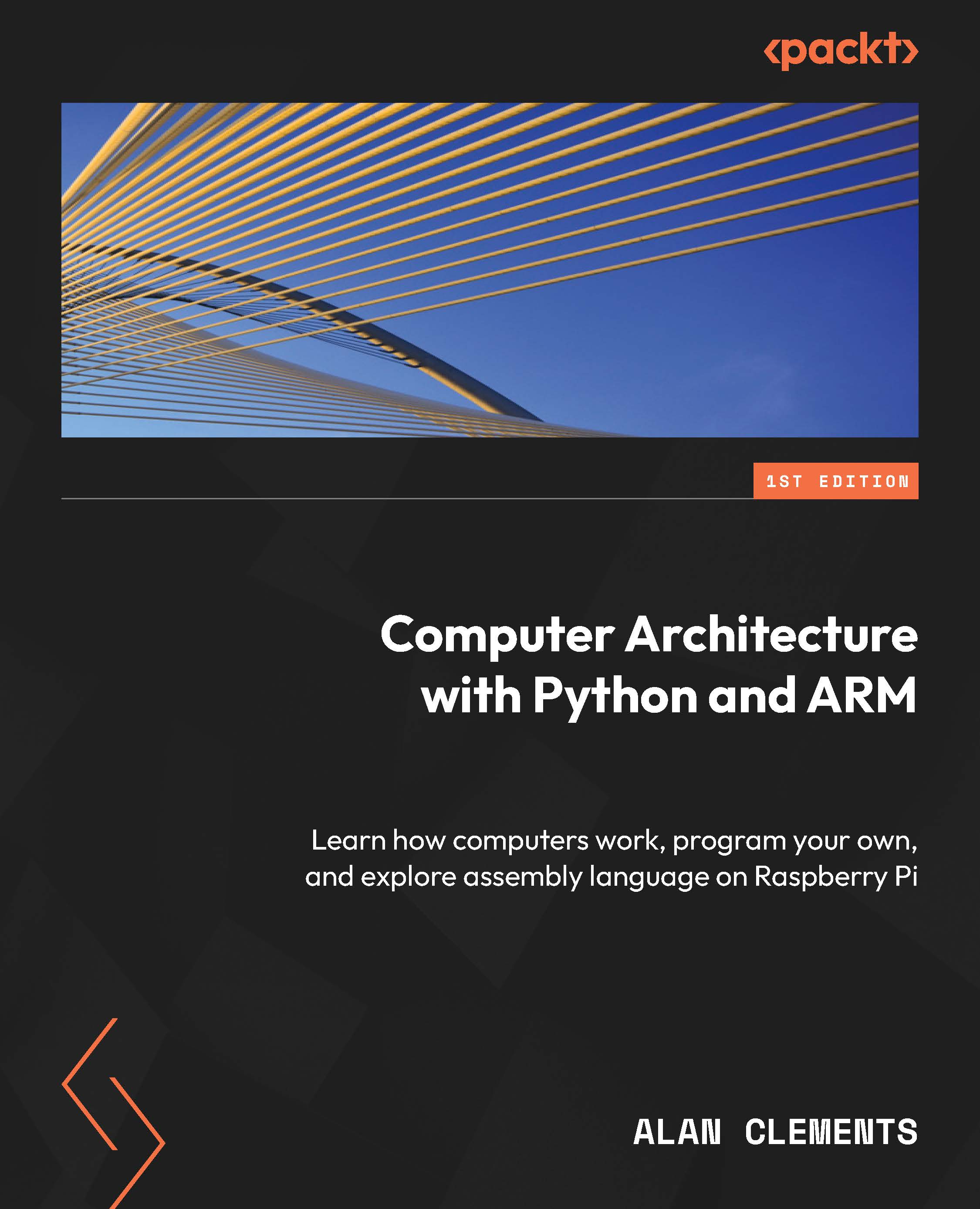
Computer Architecture with Python and ARM

Computer Architecture with Python and ARM: Learn how computers work, program your own, and explore assembly language on Raspberry Pi

eBook
€8.99 €23.99
Paperback
€29.99
Subscription
Free Trial
Renews at €18.99p/m

What do you get with Print?

Product feature icon Instant access to your digital eBook copy whilst your Print order is Shipped
Product feature icon Paperback book shipped to your preferred address
Product feature icon Download this book in EPUB and PDF formats
Product feature icon Access this title in our online reader with advanced features
Product feature icon DRM FREE - Read whenever, wherever and however you want
Product feature icon AI Assistant (beta) to help accelerate your learning
OR
Modal Close icon
Payment Processing...
tick Completed

Shipping Address

Billing Address

Shipping Methods
Table of content icon View table of contents Preview book icon Preview Book

Computer Architecture with Python and ARM

1

From Finite State Machines to Computers

In this chapter, you will discover the fundamental nature of computers. Our goal is to explain what makes a computer a computer. These concepts are important because you can’t understand how a computer works until you appreciate the implications of its sequential nature.

Once we’ve introduced the concept of digital systems, the next chapter will demonstrate how a computer operates by fetching instructions from memory and executing them. After that, we will introduce Python and demonstrate how you can write a program to simulate a computer and observe its operations. This book is all about learning by doing; by building a computer with software, you will learn how it operates and how to extend and modify it.

The remainder of this book will look at a real computer, a Raspberry Pi, and show you how to write programs for it and observe their execution. In doing so, we will move on from simulating a hypothetical computer to learning about a real computer.

A computer is a deterministic symbol processing machine. But what does that mean? Deterministic tells us that a computer always behaves in the same way when operating under the same conditions (that is, programs and inputs). If you use a computer to evaluate 2, you will always get the same result, no matter how many times you perform the operation. Not all systems are deterministic – if you toss a coin, the sequence of heads and tails is not predictable.

When we say that a computer is a symbol processing machine, we mean that it takes in symbols and operates on them to provide new symbols as an output. These symbols are anything that can be represented in digital form: letters, words, numbers, images, sound, and video. Consider a computer that’s playing chess. The input symbols that are received by the program correspond to the moves made by a player. The program operates on the input symbols according to a set of rules and produces an output symbol – the computer’s move.

Although we’ve just provided a theoretical definition of a computer, it is important to appreciate that programming involves translating information in the real world into symbols that can be manipulated by a computer – writing a set of rules (that is, a program) that tells the computer how to manipulate the symbols, and then converting the output symbols into a form that is meaningful to a human. The symbols that are processed by a computer have no intrinsic meaning to the computer – a certain pattern of bits (that is, the symbol) might represent a number, a name, a move in a game, and so on. The computer processes these bits to produce a new pattern of bits (that is, an output symbol) that has a meaning only to the programmer or user.

We are going to pose a simple problem and then solve it. Our solution will lead us to the concepts of algorithms and computers, and also introduce key concepts such as discrete digital operations, memory and storage, variables, and conditional operations. By doing this, we can determine the types of operations a computer needs to perform to solve a problem. After this, we can ask, “How can we automate this? That is, how can we build a computer?”

It’s a trite statement, but once you understand a problem, you’re well on the way to finding a solution. When you first encounter a problem that requires an algorithmic solution, you have to think about what you want to do, rather than how you are going to do it. The worst approach to problem solving is to start writing an algorithm (or even actual computer code) before you have fully explored the problem. Suppose you were asked to design a cruise control system for an automobile. In principle, this is a very simple problem with an equally simple solution:

IF cruise control on THEN keep speed constant
                     ELSE read the position of the gas pedal

Couldn’t be simpler, could it? Well, what happens if you’ve selected cruise control and someone pulls out in front of you? You could brake, but this algorithm would attempt to keep the speed constant while you are braking by applying full throttle at the same time. Alternatively, you might suggest that the act of braking should disengage the cruise control mechanism. But is the cruise control to be disengaged permanently, or should the automobile accelerate to its previous speed once the braking action has ceased? You have to think about all the aspects of the problem.

Even if you design a correct algorithm, you have to consider the effect erroneous or spurious data will have on your system. One of the most popular criticisms of computers is that they produce meaningless results if you feed them with incorrect data. This idea is summed up by the expression garbage in, garbage out (GIGO). A well-constructed algorithm should detect and filter out any garbage in the input data stream.

In this chapter, we will introduce the following topics:

  • The finite state machine
  • Solving a problem algorithmically

Technical requirements

The finite state machine

There are remarkably few fundamental concepts that you need to know about to understand what a digital computer does and how it operates. One of the most important concepts is discrete, which lies at the heart of both computer operation and computer programs.

Computers operate on discrete data elements – that is, elements whose values are chosen from a fixed and finite range of values. We use discrete values in everyday life – for example, the letters of the Roman alphabet that belong to the set {A...Z}. A letter is never between two possible values. It’s the same with the days of the week; you can have one of seven days, but you can’t have a day that is slightly Monday or just a little bit bigger than Wednesday. In the case of computers, the fundamental data element is the bit, which can only have values of 0 or 1, and all its data structures are represented by strings of 1s and 0s.

As well as discrete data values, we can have discrete points in time. Imagine that time moves in one direction, from one discrete point to another discrete point. Nothing exists between two discrete points in time. It’s a bit like a digital clock that goes from 12:15:59 to 12:16:00. There’s nothing in between.

Now, imagine state space, which is a grandiose term for all the states a system can be in (for example, a plane can be in the climbing, descending, or level flight state). States are a bit like time, except that you can go forward or backward between discrete points in state space. If there are a limited number of possible states, a device that models the transitions between states is called a finite state machine (FSM). An elevator is a finite state machine: it has states (position at the floors, doors open or closed, and so on) and inputs (the elevator call buttons, floor selection buttons, and door open and close buttons).

Before we take a serious look at FSMs, let’s begin with a simple example of how to use FSMs to describe a real system. Consider the TV of yesterday, which is a device with two states: on and off. It is always in one of these two states, and it can move between these states. It is never in a state that is neither on nor off. Modern TVs often have three states – on, standby, and off– where the standby state provides a fast-on mechanism (that is, part of the electronics is in an active on state, but the display and sound system are powered down). The standby state is often called the sleep state or idle state. We can model discrete states using a diagram. Each state is represented by a labeled circle, as demonstrated in Figure 1.1:

Figure 1.1 – Representing the three states of a television

Figure 1.1 – Representing the three states of a television

Figure 1.1 shows the three states, but it doesn’t tell us the most important information we need to know: how we move between states. We can do this by drawing lines between states and labeling them with the event that triggers a change of state. Figure 1.2 does this. Please note that we are going to construct an incorrect system first to illustrate some of the concepts concerning FSMs:

Figure 1.2 – Representing the states of a television with transitions

Figure 1.2 – Representing the states of a television with transitions

In Figure 1.2, we labeled each transition by the event that triggers it; in each case, it’s pressing a button on the remote controller. To go from off to on, you have to first press the standby button and then the on button. To go between on and standby, you must press the on button or the standby button.

We’ve forgotten something – what if you are already in a state and you press the same button? For example, let’s say the TV is on, and you press the on button. Also, what’s the initial state? Figure 1.3 rectifies these omissions.

Figure 1.3 has two innovations. There is an arrow to the off state marked Power on. This line indicates the state the system enters when you first plug it into the electricity supply. The second innovation in Figure 1.3 is that each state has a loop back to itself; for example, if you are in the on state and you press the on button, you remain in that state:

Figure 1.3 – The TV control with initialization

Figure 1.3 – The TV control with initialization

The state diagram shown in Figure 1.3 has both a logical error and an ergonomic error. What happens if you are in the off state and press the on button? If you are in the off state, pressing the on button (in this system) is incorrect because you have to go to standby first. Figure 1.4 corrects this error by dealing with incorrect inputs:

Figure 1.4 – The TV control with wrong button correction

Figure 1.4 – The TV control with wrong button correction

Figure 1.4 now provides correct operations from any state and includes the effect of pressing buttons that cause no change of state. But we still have the ergonomic error – that is, it’s a correct design that behaves in a way that many would consider poor. The standby state is a convenience that speeds up operations. However, the user does not need to know about this state – it should be invisible to the user.

Figure 1.5 demonstrates the final version of the controller. We’ve eliminated a standby button, but not the standby state. When the user presses the on button, the system goes directly to the on state. However, when the user presses off when in the on state, the system goes to the standby state. From the standby state, pressing the on button results in the power on state, while pressing off results in the power off state. Note that the same action (pressing off) can have different effects, depending on the current state:

Figure 1.5 – The TV control with a hidden standby state

Figure 1.5 – The TV control with a hidden standby state

We’ve labored with this example because the notion of FSMs is at the heart of all digital systems. All digital systems, apart from the most trivial, move from state to state, depending on the current input and past states. In a digital computer, the change-of-state trigger is the system clock. A modern computer operating at a clock speed of 4 GHz changes state every 0.25 x 10⁻⁹ s or every 0.25 ns. Light traveling at 300,000 km/s (186,000 mph) moves about 7.5 cm or 3 inches during a clock cycle.

Traffic lights example

Let’s look at a second example of an FSM. A classic example of an FSM is traffic lights at a crossroads. Consider an intersection with traffic moving north-south or east-west. The traffic may move in only one direction at a time. Assume that this is a system with a clock and a change of state is permitted every minute:

Current State of the Lights

Traffic in the North-South Direction

Traffic in the East-West Direction

Action to Be Taken On the Next Clock

Next State of the Lights

North-south

None

None

No traffic, no change

North-south

North-south

None

One or more

East-west, forces change

East-west

North-south

One or more

None

North-south, no change

North-south

North-south

One or more

One or more

East-west, forces change

East-west

East-west

None

None

No traffic, no change

East-west

East-west

None

One or more

East-west, no change

East-west

East-west

One or more

None

North-south, forces change

North-south

East-west

One or more

One or more

North-south, forces change

North-south

Table 1.1 – Traffic lights sequence table

Suppose the traffic is currently flowing north-south. At the next clock, it may either remain flowing north-south or the lights may change to allow east-west traffic. Similarly, if traffic is flowing east-west, at the next clock, it may either remain flowing east-west or the lights may change to permit north-south traffic.

We can use Table 1.1 to describe this system. We have provided the current state of the lights (direction of traffic flow), indicated whether any traffic had been detected in either the north-south or east-west direction, the action to be taken at the next clock, and the next state. The traffic rule is simple: the lights remain in their current state unless there is pending traffic in the other direction.

We can now convert this table into the FSM diagram shown in Figure 1.6. Note that we have made the east-west state the power on state; this is an arbitrary choice:

Figure 1.6 – A finite state machine for Table 1.1

Figure 1.6 – A finite state machine for Table 1.1

What have we learned? The most important point is that a system is, at any instant, in a particular state and that a transition to another state (or a transition back to the current state) is made according to a defined set of conditions. The FSM has several advantages, both as a teaching tool and a design tool:

  • It uses a simple intuitive diagram to describe a system with discrete states
  • The state transition diagram (if correct) provides a complete and unambiguous way of describing a system
  • The FSM is also an abstract machine in the sense that it models a real system, but we don’t have to worry about how the FSM is implemented in real hardware or software
  • Any FSM can be implemented either in hardware or software; that is, if you can define a state diagram on paper, you can build the circuit in dedicated hardware or write the program to run on a general-purpose computer

I have included a brief introduction to FSMs because they can be considered a precursor to the digital computer. An FSM is designed to carry out a specific task; this is built into its hardware. A computer has some of the characteristics of an FSM but you can program the transitions between states.

Solving a simple problem algorithmically

Now that we’ve introduced FSMs, we will describe a problem, solve it, and then construct our computer. A bag contains a mixture of red and white tokens. Suppose that we take a token at a time out of the bag and continue until we have removed three consecutive red tokens. We want to construct an algorithm that tells us to stop removing tokens from the bag when three reds in a row have been detected.

Before creating an algorithm, we’ll provide an FSM for this problem:

Figure 1.7 – FSM for a three-token detector

Figure 1.7 – FSM for a three-token detector

As you can see, there are four states. We begin in state S0. Each time a token is received, we move to the next state if it’s red, and back to the initial state if it’s white. Once we’ve reached state S3, the process ends. Now, we’ll perform the same operation algorithmically.

If a white token is represented by the symbol W, and a red token by R, a possible sequence of tokens might be RRWRWWWWRWWRRR (the sequence is terminated by the three Rs). An algorithm that tells us when to stop removing tokens can be written in the following form:

  • Line 1: Get a token from the bag
  • Line 2: If the token is white, then go back to line 1
  • Line 3: Get a token from the bag
  • Line 4: If the token is white, then go back to Line 1
  • Line 5: Get a token from the bag
  • Line 6: If the token is white, then go back to Line 1
  • Line 7: Success – three consecutive red tokens have been taken out of the bag

As you can see, the algorithm is expressed in plain English. It is read from top to bottom, line by line, and the action specified by each line is carried out before the next line is processed. In this algorithm, each line has a unique name (that is, Line 1, Line 2, and so on). Labeling a line enables us to refer to it; for example, when the algorithm states that we must go back to Line 1, this means that the next step to be carried out is specified by Line 1, and we continue carrying out actions from Line 1 onward. This algorithm is not entirely satisfactory – we haven’t checked that the bag contains only red and white tokens, and we haven’t dealt with the situation in which we run out of tokens before we locate the sequence we’re looking for. At the moment, we are not concerned with these details.

There’s no single solution to this problem – more often than not, lots of algorithms can be constructed to solve a given problem. Let’s derive another algorithm to detect a sequence of three consecutive red tokens:

Line 1: Set the total number of consecutive red tokens found so far to 0

Line 2: Get a token from the bag

Line 3: If the token is white, then go back to Line 1

Line 4: Add 1 to the number of consecutive red tokens found so far

Line 5: If the number of consecutive red tokens is less than 3, then go back to Line 2

Line 6: Success – 3 consecutive red tokens have been taken out of the bag

This algorithm is more versatile because it can easily be modified to detect any number of consecutive red tokens simply by changing the value of 3 in Line 5 of the algorithm.

Figure 1.8 presents this algorithm diagrammatically in the form of a flowchart that shows the sequence of operations that take place when executing an algorithm. Lines with arrowheads indicate the sequence in which operations are carried out. Boxes indicate the actions themselves, and diamonds represent conditional actions. The expression in the diamond is evaluated to yield either “yes” or “no,” and control flows in one direction or another. In general, flowcharts are well suited to depicting simple algorithms, but they are regarded as very unsuitable for complex algorithms. A flowchart for a complex algorithm looks like a bowl of spaghetti – but without the spaghetti’s inherent clarity and organization.

Figure 1.8 – An algorithm represented by a flowchart

Figure 1.8 – An algorithm represented by a flowchart

Constructing an algorithm

The next step is to provide an algorithm that tells us how to solve this problem clearly and unambiguously. As we step through the sequence of digits, we will need to keep track of what’s happening, as Table 1.2 demonstrates:

Position in sequence

0

1

2

3

4

5

6

7

8

9

10

11

12

13

New token

R

R

W

R

W

W

W

W

R

W

W

R

R

R

Is it red?

Y

Y

N

Y

N

N

N

N

Y

N

N

Y

Y

Y

Number of reds

1

2

0

1

0

0

0

0

1

0

0

1

2

3

Table 1.2 – A sequence of tokens selected at random

Pseudocode is a term that’s applied to a method of expressing an algorithm in something that falls between plain English and a formal programming language. The following pseudocode expresses the actions we need to perform. The initialization operations that we perform once at the beginning are in normal typeface, while the repetitive actions defined by REPEAT...UNTIL are in bold. We will look at these operations in detail when we introduce Python:

1.    Set numRed to 0
2.    Set maxRed to 3
3.    REPEAT
4.        Get a token
5.        IF its color is red
6.        THEN numRed = numRed + 1
7.        ELSE numRed = 0
8.    UNTIL numRed = maxRed

This pseudocode employs two constructs found in many high-level computer languages: the REPEAT...UNTIL construct in lines 3 to 8, and the IF...THEN...ELSE construct on lines 5 to 7. REPEAT...UNTIL lets you carry out an action one or more times, while IF...THEN...ELSE lets you choose between one of two possible courses of action.

The IF...THEN...ELSE construct is central to the operation of digital computers and you will encounter it many times in this book.

The next step is to introduce Python so that we can write a program to implement this algorithm. Then, we can start to look at the computer. The following code shows a Python program and its output when executed. We haven’t introduced Python yet. The purpose of this program is to demonstrate how close it is to the preceding algorithm and the simplicity of Python:

Sequence =['W','R','R','W','R','W','W','W','W','R','W','W','R','R','R']
numRed = 0
maxRed = 3
count  = 0
while numRed != maxRed:
    token = sequence[count]
    if token == 'R':
        numRed = numRed + 1
    else: numRed = 0
    print('count', count,'token',token,'numRed',numRed)
    count = count + 1
print('Three reds found starting at location', count - 3)

The while numRed != maxRed: line means carry out the block of indented operations, so long as (while) the value of numRed is not equal to maxRed. The != Python operator means not equal.

This is the output when the program is executed. It correctly identifies three consecutive reds and indicates the location of the first run in the run of three:

count  0 token  W numRed 0
count  1 token  R numRed 1
count  2 token  R numRed 2
count  3 token  W numRed 0
count  4 token  R numRed 1
count  5 token  W numRed 0
count  6 token  W numRed 0
count  7 token  W numRed 0
count  8 token  W numRed 0
count  9 token  R numRed 1
count 10 token  W numRed 0
count 11 token  W numRed 0
count 12 token  R numRed 1
count 13 token  R numRed 2
count 14 token  R numRed 3
Three reds found starting at location 12

Summary

In this first chapter, we introduced the concept of a computer via an FSM. A state machine is an abstraction of any system that can exist in one of several states at any instant. State machines are defined in terms of the states and the transitions between states. We introduced state machines as a precursor to digital systems. State machines introduce the notion of discrete states and discrete times. A state machine moves from one state to another at discrete instants in time. This mirrors the action of a program where actions (change of state) take place only when an instruction is executed.

State machines can model systems as simple as traffic lights to a game of chess or a computer program. We also introduced the idea of algorithms – that is, a set of rules used to solve a problem. Later in this book, we’ll explain how computers can implement algorithms.

In Chapter 2, we’ll provide a brief overview of n. We’ve chosen this language because it has a remarkably shallow learning curve, is very powerful (it does a lot with a few lines of code), is taught in many universities, and is freely available to run on PCs, Macs, and Raspberry Pi systems.

Left arrow icon Right arrow icon
Download code icon Download Code

Key benefits

  • Build a computer simulator with Python: Learn computer architecture by designing and constructing a simulator
  • Python for architecture: Use Python to simulate and execute assembly language instructions
  • ARM programming on Raspberry Pi: Explore ARM assembly language and run programs on Raspberry Pi

Description

This comprehensive guide offers a unique and immersive learning experience by combining Python programming with ARM architecture. Starting with an introduction to computer architecture and the flow of data within a computer system, you’ll progress to building your own interpreter using Python. You’ll see how this foundation enables the simulation of computer operations and learn ways to enhance a simulator by adding new instructions and displaying improved results. As you advance, you’ll explore the TC1 Assembler and Simulator Program to gain insights into instruction analysis and explore practical examples of simulators. This will help you build essential skills in understanding complex computer instructions, strengthening your grasp of computer architecture. Moreover, you’ll be introduced to the Raspberry Pi operating system, preparing you to delve into the detailed language of the ARM computer. This includes exploring the ARM instruction set architecture, data-processing instructions, subroutines, and the stack. With clear explanations, practical examples, and coding exercises, this resource will enable you to design and construct your own computer simulator, simulate assembly language programs, and leverage the Raspberry Pi for ARM programming.

Who is this book for?

This book is for university students studying computer science, particularly those enrolled in a computer architecture module. With its practical approach and succinct explanations, it is also suitable for hobbyists, enthusiasts, and self-learners seeking a deeper understanding of computer systems. The book assumes foundational knowledge of number bases, binary arithmetic, and Boolean logic concepts. While it primarily caters to the computer science field, this book is less geared toward electrical or electronics engineering.

What you will learn

  • Master the core principles of computer architecture
  • Understand the role of registers, memory, and data flow in computers
  • Discover how to design and implement a computer simulator using Python
  • Simulate and execute assembly language programs on the simulator
  • Enhance the simulator using new instructions for improved output
  • Analyze complex computer instructions for deeper architectural understanding
  • Explore the ARM instruction set and data processing on the Raspberry Pi
  • Develop proficiency in writing, assembling, and running ARM code on the Raspberry Pi
Estimated delivery fee Deliver to Lithuania

Premium delivery 7 - 10 business days

€25.95
(Includes tracking information)

Product Details

Country selected
Publication date, Length, Edition, Language, ISBN-13
Publication date : Jul 31, 2023
Length: 412 pages
Edition : 1st
Language : English
ISBN-13 : 9781837636679
Category :
Languages :

What do you get with Print?

Product feature icon Instant access to your digital eBook copy whilst your Print order is Shipped
Product feature icon Paperback book shipped to your preferred address
Product feature icon Download this book in EPUB and PDF formats
Product feature icon Access this title in our online reader with advanced features
Product feature icon DRM FREE - Read whenever, wherever and however you want
Product feature icon AI Assistant (beta) to help accelerate your learning
OR
Modal Close icon
Payment Processing...
tick Completed

Shipping Address

Billing Address

Shipping Methods
Estimated delivery fee Deliver to Lithuania

Premium delivery 7 - 10 business days

€25.95
(Includes tracking information)

Product Details

Publication date : Jul 31, 2023
Length: 412 pages
Edition : 1st
Language : English
ISBN-13 : 9781837636679
Category :
Languages :

Packt Subscriptions

See our plans and pricing
Modal Close icon
€18.99 billed monthly
Feature tick icon Unlimited access to Packt's library of 7,000+ practical books and videos
Feature tick icon Constantly refreshed with 50+ new titles a month
Feature tick icon Exclusive Early access to books as they're written
Feature tick icon Solve problems while you work with advanced search and reference features
Feature tick icon Offline reading on the mobile app
Feature tick icon Simple pricing, no contract
€189.99 billed annually
Feature tick icon Unlimited access to Packt's library of 7,000+ practical books and videos
Feature tick icon Constantly refreshed with 50+ new titles a month
Feature tick icon Exclusive Early access to books as they're written
Feature tick icon Solve problems while you work with advanced search and reference features
Feature tick icon Offline reading on the mobile app
Feature tick icon Choose a DRM-free eBook or Video every month to keep
Feature tick icon PLUS own as many other DRM-free eBooks or Videos as you like for just €5 each
Feature tick icon Exclusive print discounts
€264.99 billed in 18 months
Feature tick icon Unlimited access to Packt's library of 7,000+ practical books and videos
Feature tick icon Constantly refreshed with 50+ new titles a month
Feature tick icon Exclusive Early access to books as they're written
Feature tick icon Solve problems while you work with advanced search and reference features
Feature tick icon Offline reading on the mobile app
Feature tick icon Choose a DRM-free eBook or Video every month to keep
Feature tick icon PLUS own as many other DRM-free eBooks or Videos as you like for just €5 each
Feature tick icon Exclusive print discounts

Frequently bought together


Stars icon
Total 105.97
Computer Architecture with Python and ARM
€29.99
A Handbook of Mathematical Models with Python
€37.99
50 Algorithms Every Programmer Should Know
€37.99
Total 105.97 Stars icon
Banner background image

Table of Contents

16 Chapters
Part 1: Using Python to Simulate a Computer Chevron down icon Chevron up icon
Chapter 1: From Finite State Machines to Computers Chevron down icon Chevron up icon
Chapter 2: High-Speed Introduction to Python Chevron down icon Chevron up icon
Chapter 3: Data Flow in a Computer Chevron down icon Chevron up icon
Chapter 4: Crafting an Interpreter – First Steps Chevron down icon Chevron up icon
Chapter 5: A Little More Python Chevron down icon Chevron up icon
Chapter 6: TC1 Assembler and Simulator Design Chevron down icon Chevron up icon
Chapter 7: Extending the TC1 Chevron down icon Chevron up icon
Chapter 8: Simulators for Other Architectures Chevron down icon Chevron up icon
Part 2: Using Raspberry Pi to Study a Real Computer Architecture Chevron down icon Chevron up icon
Chapter 9: Raspberry Pi: An Introduction Chevron down icon Chevron up icon
Chapter 10: A Closer Look at the ARM Chevron down icon Chevron up icon
Chapter 11: ARM Addressing Modes Chevron down icon Chevron up icon
Chapter 12: Subroutines and the Stack Chevron down icon Chevron up icon
Index Chevron down icon Chevron up icon
Other Books You May Enjoy Chevron down icon Chevron up icon

Customer reviews

Top Reviews
Rating distribution
Full star icon Full star icon Full star icon Full star icon Half star icon 4.6
(7 Ratings)
5 star 57.1%
4 star 42.9%
3 star 0%
2 star 0%
1 star 0%
Filter icon Filter
Top Reviews

Filter reviews by


POE Sep 12, 2023
Full star icon Full star icon Full star icon Full star icon Full star icon 5
This book is organized into two parts. The first part walks us through how to use Python to simulate a computer. If you are not already familiar with Python, you will appreciate the High-Speed Introduction to Python chapter as it covers everything from soup to nuts in under 30 pages. This first part also covers instruction architecture level and von Neumann architecture to help explain how data flows in a computer. Machine -level instruction sets (CISC and RISC) are also covered.The true gem of this book, in my opinion, is that the author teaches us how to build a simple computer interpreter in Python. Even if you only want to further your Python knowledge and are not interested in computer architecture, this is a great resource.The second main section of the book covers the use of a Raspberry Pi for studying computer architecture. The author does a great job in getting readers up to speed quickly with Raspberry Pi operations. If you follow the examples in the book, you will install and configure programs and packages, write assembly language code, and assemble ARM code. Troubleshooting and debugging are also covered. This section dives deep into ARM architecture, operations, addressing, and subroutines.
Amazon Verified review Amazon
arsalan Sep 04, 2023
Full star icon Full star icon Full star icon Full star icon Full star icon 5
This book is a valuable resource for individuals eager to explore the inner workings of computers and develop practical programming skills. Author offers a solid foundation in computer architecture, coupled with hands-on exercises that reinforce learning. This book provides a fantastic starting point for enthusiasts and students looking to delve into the fascinating world of computer architecture and ARM programming.
Amazon Verified review Amazon
Deborah Scherrer Oct 28, 2023
Full star icon Full star icon Full star icon Full star icon Full star icon 5
This excellent book, written by a skilled author, explains how a computer works by teaching us, step by step, how to build a simple computer interpreter in Python. Designed to support teaching the basics of computer architecture, it is essentially a combination of sections on computer architecture, Python, and Raspberry Pi, in depth. We learn-by-doing as Clements walks us through finite state machines, data flow, interpreters, instruction sets, and simulators - culminating by producing our own interpreter. Examples and code are freely available on GitHub.Although this would be a good textbook for computer architect students, it is also valuable for someone who wants to understand how computers work in detail. Raspberry PI users and those wanting to learn Python could benefit. Even software engineers might use it to better understand how computer architecture relates to efficiency, security, and such.Clements is an excellent educator – entirely knowledgeable on the subject. He teaches hands-on by example – “learn by doing”. The concepts and terms are explained well, in depth, and illustrations provided to help comprehension. No small feat given the nature of the subjects.Had I been the author, I might have divided the book into two, using the Raspberry Pi/ARM section as a follow-on. However, the volume is well-written, full and with complete explanations. Comprehensive and extensive, it’ll take you a while to get through it. But if you’re game, this is an excellent learning tool. Wish I had had it at the start of my career!
Amazon Verified review Amazon
Amazon Customer Sep 20, 2023
Full star icon Full star icon Full star icon Full star icon Full star icon 5
Alan Clements is a pioneer in the industry and has, yet again, authored an excellent recipe book that reads like a novel. It is detailed, clear, concise, and to the point.I felt like the author was sitting beside me looking over my shoulder and answering my questions before I asked them.The book gets you up and running with Python, ARM, and the Pi quickly and efficiently with what you need to know and allows students to move as fast as they want through the material while learning and combining the different parts.The relevant and essential content was bounded and described in perfect ratios: not too lengthy and voluminous while not too short and brief. Every bit of information was useful and left just enough to my imagination to keep me engaged.An abundance of sample and example code including clear explanations of what, where, why, and how. Clear descriptions of all resources, code, and everything you need to get up and running quickly.A valuable source to design custom platforms combining elements of RISC, CISC, Von-Neumann, and non-Von-Neumann architectures. An excellent cross section of relevant, scalable, and useful material.Pay close attention to the material. It is designed to be immediately referenced, applied, and/or built upon.
Amazon Verified review Amazon
D&A Sep 05, 2023
Full star icon Full star icon Full star icon Full star icon Empty star icon 4
Commencing with an exploration of computer architecture and the intricate pathways of data within a computer system, you will advance to the creation of your very own interpreter using Python. This solid foundation will empower you to simulate computer operations, providing you with the tools to enhance your simulator by introducing new instructions and showcasing improved outcomes. Abundant with lucid explanations, hands-on examples, and coding exercises, this invaluable resource equips you with the skills to design and construct your personalized computer simulator, simulate assembly language programs effectively, and harness the potential of Raspberry Pi for ARM programming.
Amazon Verified review Amazon
Get free access to Packt library with over 7500+ books and video courses for 7 days!
Start Free Trial

FAQs

What is the delivery time and cost of print book? Chevron down icon Chevron up icon

Shipping Details

USA:

'

Economy: Delivery to most addresses in the US within 10-15 business days

Premium: Trackable Delivery to most addresses in the US within 3-8 business days

UK:

Economy: Delivery to most addresses in the U.K. within 7-9 business days.
Shipments are not trackable

Premium: Trackable delivery to most addresses in the U.K. within 3-4 business days!
Add one extra business day for deliveries to Northern Ireland and Scottish Highlands and islands

EU:

Premium: Trackable delivery to most EU destinations within 4-9 business days.

Australia:

Economy: Can deliver to P. O. Boxes and private residences.
Trackable service with delivery to addresses in Australia only.
Delivery time ranges from 7-9 business days for VIC and 8-10 business days for Interstate metro
Delivery time is up to 15 business days for remote areas of WA, NT & QLD.

Premium: Delivery to addresses in Australia only
Trackable delivery to most P. O. Boxes and private residences in Australia within 4-5 days based on the distance to a destination following dispatch.

India:

Premium: Delivery to most Indian addresses within 5-6 business days

Rest of the World:

Premium: Countries in the American continent: Trackable delivery to most countries within 4-7 business days

Asia:

Premium: Delivery to most Asian addresses within 5-9 business days

Disclaimer:
All orders received before 5 PM U.K time would start printing from the next business day. So the estimated delivery times start from the next day as well. Orders received after 5 PM U.K time (in our internal systems) on a business day or anytime on the weekend will begin printing the second to next business day. For example, an order placed at 11 AM today will begin printing tomorrow, whereas an order placed at 9 PM tonight will begin printing the day after tomorrow.


Unfortunately, due to several restrictions, we are unable to ship to the following countries:

  1. Afghanistan
  2. American Samoa
  3. Belarus
  4. Brunei Darussalam
  5. Central African Republic
  6. The Democratic Republic of Congo
  7. Eritrea
  8. Guinea-bissau
  9. Iran
  10. Lebanon
  11. Libiya Arab Jamahriya
  12. Somalia
  13. Sudan
  14. Russian Federation
  15. Syrian Arab Republic
  16. Ukraine
  17. Venezuela
What is custom duty/charge? Chevron down icon Chevron up icon

Customs duty are charges levied on goods when they cross international borders. It is a tax that is imposed on imported goods. These duties are charged by special authorities and bodies created by local governments and are meant to protect local industries, economies, and businesses.

Do I have to pay customs charges for the print book order? Chevron down icon Chevron up icon

The orders shipped to the countries that are listed under EU27 will not bear custom charges. They are paid by Packt as part of the order.

List of EU27 countries: www.gov.uk/eu-eea:

A custom duty or localized taxes may be applicable on the shipment and would be charged by the recipient country outside of the EU27 which should be paid by the customer and these duties are not included in the shipping charges been charged on the order.

How do I know my custom duty charges? Chevron down icon Chevron up icon

The amount of duty payable varies greatly depending on the imported goods, the country of origin and several other factors like the total invoice amount or dimensions like weight, and other such criteria applicable in your country.

For example:

  • If you live in Mexico, and the declared value of your ordered items is over $ 50, for you to receive a package, you will have to pay additional import tax of 19% which will be $ 9.50 to the courier service.
  • Whereas if you live in Turkey, and the declared value of your ordered items is over € 22, for you to receive a package, you will have to pay additional import tax of 18% which will be € 3.96 to the courier service.
How can I cancel my order? Chevron down icon Chevron up icon

Cancellation Policy for Published Printed Books:

You can cancel any order within 1 hour of placing the order. Simply contact customercare@packt.com with your order details or payment transaction id. If your order has already started the shipment process, we will do our best to stop it. However, if it is already on the way to you then when you receive it, you can contact us at customercare@packt.com using the returns and refund process.

Please understand that Packt Publishing cannot provide refunds or cancel any order except for the cases described in our Return Policy (i.e. Packt Publishing agrees to replace your printed book because it arrives damaged or material defect in book), Packt Publishing will not accept returns.

What is your returns and refunds policy? Chevron down icon Chevron up icon

Return Policy:

We want you to be happy with your purchase from Packtpub.com. We will not hassle you with returning print books to us. If the print book you receive from us is incorrect, damaged, doesn't work or is unacceptably late, please contact Customer Relations Team on customercare@packt.com with the order number and issue details as explained below:

  1. If you ordered (eBook, Video or Print Book) incorrectly or accidentally, please contact Customer Relations Team on customercare@packt.com within one hour of placing the order and we will replace/refund you the item cost.
  2. Sadly, if your eBook or Video file is faulty or a fault occurs during the eBook or Video being made available to you, i.e. during download then you should contact Customer Relations Team within 14 days of purchase on customercare@packt.com who will be able to resolve this issue for you.
  3. You will have a choice of replacement or refund of the problem items.(damaged, defective or incorrect)
  4. Once Customer Care Team confirms that you will be refunded, you should receive the refund within 10 to 12 working days.
  5. If you are only requesting a refund of one book from a multiple order, then we will refund you the appropriate single item.
  6. Where the items were shipped under a free shipping offer, there will be no shipping costs to refund.

On the off chance your printed book arrives damaged, with book material defect, contact our Customer Relation Team on customercare@packt.com within 14 days of receipt of the book with appropriate evidence of damage and we will work with you to secure a replacement copy, if necessary. Please note that each printed book you order from us is individually made by Packt's professional book-printing partner which is on a print-on-demand basis.

What tax is charged? Chevron down icon Chevron up icon

Currently, no tax is charged on the purchase of any print book (subject to change based on the laws and regulations). A localized VAT fee is charged only to our European and UK customers on eBooks, Video and subscriptions that they buy. GST is charged to Indian customers for eBooks and video purchases.

What payment methods can I use? Chevron down icon Chevron up icon

You can pay with the following card types:

  1. Visa Debit
  2. Visa Credit
  3. MasterCard
  4. PayPal
What is the delivery time and cost of print books? Chevron down icon Chevron up icon

Shipping Details

USA:

'

Economy: Delivery to most addresses in the US within 10-15 business days

Premium: Trackable Delivery to most addresses in the US within 3-8 business days

UK:

Economy: Delivery to most addresses in the U.K. within 7-9 business days.
Shipments are not trackable

Premium: Trackable delivery to most addresses in the U.K. within 3-4 business days!
Add one extra business day for deliveries to Northern Ireland and Scottish Highlands and islands

EU:

Premium: Trackable delivery to most EU destinations within 4-9 business days.

Australia:

Economy: Can deliver to P. O. Boxes and private residences.
Trackable service with delivery to addresses in Australia only.
Delivery time ranges from 7-9 business days for VIC and 8-10 business days for Interstate metro
Delivery time is up to 15 business days for remote areas of WA, NT & QLD.

Premium: Delivery to addresses in Australia only
Trackable delivery to most P. O. Boxes and private residences in Australia within 4-5 days based on the distance to a destination following dispatch.

India:

Premium: Delivery to most Indian addresses within 5-6 business days

Rest of the World:

Premium: Countries in the American continent: Trackable delivery to most countries within 4-7 business days

Asia:

Premium: Delivery to most Asian addresses within 5-9 business days

Disclaimer:
All orders received before 5 PM U.K time would start printing from the next business day. So the estimated delivery times start from the next day as well. Orders received after 5 PM U.K time (in our internal systems) on a business day or anytime on the weekend will begin printing the second to next business day. For example, an order placed at 11 AM today will begin printing tomorrow, whereas an order placed at 9 PM tonight will begin printing the day after tomorrow.


Unfortunately, due to several restrictions, we are unable to ship to the following countries:

  1. Afghanistan
  2. American Samoa
  3. Belarus
  4. Brunei Darussalam
  5. Central African Republic
  6. The Democratic Republic of Congo
  7. Eritrea
  8. Guinea-bissau
  9. Iran
  10. Lebanon
  11. Libiya Arab Jamahriya
  12. Somalia
  13. Sudan
  14. Russian Federation
  15. Syrian Arab Republic
  16. Ukraine
  17. Venezuela