Search icon CANCEL
Subscription
0
Cart icon
Your Cart (0 item)
Close icon
You have no products in your basket yet
Save more on your purchases! discount-offer-chevron-icon
Savings automatically calculated. No voucher code required.
Arrow left icon
Explore Products
Best Sellers
New Releases
Books
Videos
Audiobooks
Learning Hub
Newsletter Hub
Free Learning
Arrow right icon
timer SALE ENDS IN
0 Days
:
00 Hours
:
00 Minutes
:
00 Seconds
Building Statistical Models in Python

Building Statistical Models in Python: Develop useful models for regression, classification, time series, and survival analysis

Arrow left icon
Profile Icon Huy Hoang Nguyen Profile Icon Paul N Adams Profile Icon Stuart J Miller
Arrow right icon
€37.99
Full star icon Full star icon Full star icon Full star icon Half star icon 4.9 (11 Ratings)
Paperback Aug 2023 420 pages 1st Edition
eBook
€8.99 €29.99
Paperback
€37.99
Subscription
Free Trial
Renews at €18.99p/m
eBook
€8.99 €29.99
Paperback
€37.99
Subscription
Free Trial
Renews at €18.99p/m

What do you get with Print?

Product feature icon Instant access to your digital eBook copy whilst your Print order is Shipped
Product feature icon Colour book shipped to your preferred address
Product feature icon Download this book in EPUB and PDF formats
Product feature icon Access this title in our online reader with advanced features
Product feature icon DRM FREE - Read whenever, wherever and however you want
Product feature icon AI Assistant (beta) to help accelerate your learning
OR
Modal Close icon
Payment Processing...
tick Completed

Shipping Address

Billing Address

Shipping Methods
Table of content icon View table of contents Preview book icon Preview Book

Building Statistical Models in Python

Sampling and Generalization

In this chapter, we will describe the concept of populations and sampling from populations, including some common strategies for sampling. The discussion of sampling will lead to a section that will describe generalization. Generalization will be discussed as it relates to using samples to make conclusions about their respective populations. When modeling for statistical inference, it is necessary to ensure that samples can be generalized to populations. We will provide an in-depth overview of this bridge through the subjects in this chapter.

We will cover the following main topics:

  • Software and environment setup
  • Population versus sample
  • Population inference from samples
  • Sampling strategies – random, systematic, and stratified

Software and environment setup

Python is one of the most popular programming languages for data science and machine learning thanks to the large open source community that has driven the development of these libraries. Python’s ease of use and flexible nature made it a prime candidate in the data science world, where experimentation and iteration are key features of the development cycle. While there are new languages in development for data science applications, such as Julia, Python currently remains the key language for data science due to its wide breadth of open source projects, supporting applications from statistical modeling to deep learning. We have chosen to use Python in this book due to its positioning as an important language for data science and its demand in the job market.

Python is available for all major operating systems: Microsoft Windows, macOS, and Linux. Additionally, the installer and documentation can be found at the official website: https://www.python.org/.

This book is written for Python version 3.8 (or higher). It is recommended that you use whatever recent version of Python that is available. It is not likely that the code found in this book will be compatible with Python 2.7, and most active libraries have already started dropping support for Python 2.7 since official support ended in 2020.

The libraries used in this book can be installed with the Python package manager, pip, which is part of the standard Python library in contemporary versions of Python. More information about pip can be found here: https://docs.python.org/3/installing/index.html. After pip is installed, packages can be installed using pip on the command line. Here is basic usage at a glance:

Install a new package using the latest version:

pip install SomePackage

Install the package with a specific version, version 2.1 in this example:

pip install SomePackage==2.1

A package that is already installed can be upgraded with the --upgrade flag:

pip install SomePackage –upgrade

In general, it is recommended to use Python virtual environments between projects and to keep project dependencies separate from system directories. Python provides a virtual environment utility, venv, which, like pip, is part of the standard library in contemporary versions of Python. Virtual environments allow you to create individual binaries of Python, where each binary of Python has its own set of installed dependencies. Using virtual environments can prevent package version issues and conflict when working on multiple Python projects. Details on setting up and using virtual environments can be found here: https://docs.python.org/3/library/venv.html.

While we recommend the use of Python and Python’s virtual environments for environment setups, a highly recommended alternative is Anaconda. Anaconda is a free (enterprise-ready) analytics-focused distribution of Python by Anaconda Inc. (previously Continuum Analytics). Anaconda distributions come with many of the core data science packages, common IDEs (such as Jupyter and Visual Studio Code), and a graphical user interface for managing environments. Anaconda can be installed using the installer found at the Anaconda website here: https://www.anaconda.com/products/distribution.

Anaconda comes with its own package manager, conda, which can be used to install new packages similarly to pip.

Install a new package using the latest version:

conda install SomePackage

Upgrade a package that is already installed:

conda upgrade SomePackage

Throughout this book, we will make use of several core libraries in the Python data science ecosystem, such as NumPy for array manipulations, pandas for higher-level data manipulations, and matplotlib for data visualization. The package versions used for this book are contained in the following list. Please ensure that the versions installed in your environment are equal to or greater than the versions listed. This will help ensure that the code examples run correctly:

  • statsmodels 0.13.2
  • Matplotlib 3.5.2
  • NumPy 1.23.0
  • SciPy 1.8.1
  • scikit-learn 1.1.1
  • pandas 1.4.3

The packages used for the code in this book are shown here in Figure 1.1. The __version__ method can be used to print the package version in code.

Figure 1.1 – Package versions used in this book

Figure 1.1 – Package versions used in this book

Having set up the technical environment for the book, let’s get into the statistics. In the next sections, we will discuss the concepts of population and sampling. We will demonstrate sampling strategies with code implementations.

Population versus sample

In general, the goal of statistical modeling is to answer a question about a group by making an inference about that group. The group we are making an inference on could be machines in a production factory, people voting in an election, or plants on different plots of land. The entire group, every individual item or entity, is referred to as the population. In most cases, the population of interest is so large that it is not practical or even possible to collect data on every entity in the population. For instance, using the voting example, it would probably not be possible to poll every person that voted in an election. Even if it was possible to reach all the voters for the election of interest, many voters may not consent to polling, which would prevent collection on the entire population. An additional consideration would be the expense of polling such a large group. These factors make it practically impossible to collect population statistics in our example of vote polling. These types of prohibitive factors exist in many cases where we may want to assess a population-level attribute. Fortunately, we do not need to collect data on the entire population of interest. Inferences about a population can be made using a subset of the population. This subset of the population is called a sample. This is the main idea of statistical modeling. A model will be created using a sample and inferences will be made about the population.

In order to make valid inferences about the population of interest using a sample, the sample must be representative of the population of interest, meaning that the sample should contain the variation found in the population. For example, if we were interested in making an inference about plants in a field, it is unlikely that samples from one corner of the field would be sufficient for inferences about the larger population. There would likely be variations in plant characteristics over the entire field. We could think of various reasons why there might be variation. For this example, we will consider some examples from Figure 1.2.

Figure 1.2 – Field of plants

Figure 1.2 – Field of plants

The figure shows that Sample A is near a forest. This sample area may be affected by the presence of the forest; for example, some of the plants in that sample may receive less sunlight than plants in the other sample. Sample B is shown to be in between the main irrigation lines. It’s conceivable that this sample receives more water on average than the other two samples, which may have an effect on the plants in this sample. The final Sample C is near a road. This sample may see other effects that are not seen in Sample A or B.

If samples were only taken from one of those sections, the inferences from those samples would be biased and would not provide valid references about the population. Thus, samples would need to be taken from across the entire field to create a sample that is more likely to be representative of the population of plants. When taking samples from populations, it is critical to ensure the sampling method is robust to possible issues, such as the influence of irrigation and shade in the previous example. Whenever taking a sample from a population, it’s important to identify and mitigate possible influences of bias because biases in data will affect your model and skew your conclusions.

In the next section, various methods for sampling from a dataset will be discussed. An additional consideration is the sample size. The sample size impacts the type of statistical tools we can use, the distributional assumptions that can be made about the sample, and the confidence of inferences and predictions. The impact of sample size will be explored in depth in Chapter 2, Distributions of Data and Chapter 3, Hypothesis Testing.

Population inference from samples

When using a statistical model to make inferential conclusions about a population from a sample subset of that population, the study design must account for similar degrees of uncertainty in its variables as those in the population. This is the variation mentioned earlier in this chapter. To appropriately draw inferential conclusions about a population, any statistical model must be structured around a chance mechanism. Studies structured around these chance mechanisms are called randomized experiments and provide an understanding of both correlation and causation.

Randomized experiments

There are two primary characteristics of a randomized experiment:

  • Random sampling, colloquially referred to as random selection
  • Random assignment of treatments, which is the nature of the study

Random sampling

Random sampling (also called random selection) is designed with the intent of creating a sample representative of the overall population so that statistical models generalize the population well enough to assign cause-and-effect outcomes. In order for random sampling to be successful, the population of interest must be well defined. All samples taken from the population must have a chance of being selected. In considering the example of polling voters, all voters must be willing to be polled. Once all voters are entered into a lottery, random sampling can be used to subset voters for modeling. Sampling from only voters who are willing to be polled introduces sampling bias into statistical modeling, which can lead to skewed results. The sampling method in the scenario where only some voters are willing to participate is called self-selection. Any information obtained and modeled from self-selected samples – or any non-random samples – cannot be used for inference.

Random assignment of treatments

The random assignment of treatments refers to two motivators:

  • The first motivator is to gain an understanding of specific input variables and their influence on the response – for example, understanding whether assigning treatment A to a specific individual may produce more favorable outcomes than a placebo.
  • The second motivator is to remove the impact of external variables on the outcomes of a study. These external variables, called confounding variables (or confounders), are important to remove as they often prove difficult to control. They may have unpredictable values or even be unknown to the researcher. The consequence of including confounders is that the outcomes of a study may not be replicable, which can be costly. While confounders can influence outcomes, they can also influence input variables, as well as the relationships between those variables.

Referring back to the example in the earlier section, Population versus sample, consider a farmer who decides to start using pesticides on his crops and wants to test two different brands. The farmer knows there are three distinct areas of the land; plot A, plot B, and plot C. To determine the success of the pesticides and prevent damage to the crops, the farmer randomly chooses 60 plants from each plot (this is called stratified random sampling where random sampling is stratified across each plot) for testing. This selection is representative of the population of plants. From this selection, the farmer labels his plants (labeling doesn’t need to be random). For each plot, the farmer shuffles the labels into a bag, to randomize them, and begins selecting 30 plants. The first 30 plants get one of two treatments and the other 30 are given the other treatment. This is a random assignment of treatment. Assuming the three separate plots represent a distinct set of confounding variables on crop yield, the farmer will have enough information to obtain an inference about the crop yield for each pesticide brand.

Observational study

The other type of statistical study often performed is an observational study, in which the researcher seeks to learn through observing data that already exists. An observational study can aid in the understanding of input variables and their relationships to both the target and each other, but cannot provide cause-and-effect understanding as a randomized experiment can. An observational study may have one of the two components of a randomized experiment – either random sampling or random assignment of treatment – but without both components, will not directly yield inference. There are many reasons why an observational study may be performed versus a randomized experiment, such as the following:

  • A randomized experiment being too costly
  • Ethical constraints for an experiment (for example, an experiment to determine the rate of birth defects caused by smoking while pregnant)
  • Using data from prior randomized experiments, which thus removes the need for another experiment

One method for deriving some causality from an observational study is to perform random sampling and repeated analysis. Repeated random sampling and analysis can help minimize the impact of confounding variables over time. This concept plays a huge role in the usefulness of big data and machine learning, which has gained a lot of importance in many industries within this century. While almost any tool that can be used for observational analysis can also be used for a randomized experiment, this book focuses primarily on tools for observational analysis, as this is more common in most industries.

It can be said that statistics is a science for helping make the best decisions when there are quantifiable uncertainties. All statistical tests contain a null hypothesis and an alternative hypothesis. That is to say, an assumption that there is no statistically significant difference between data (the null hypothesis) or that there is a statistically significant difference between data (the alternative hypothesis). The term statistically significant difference implies the existence of a benchmark – or threshold – beyond which a measure takes place and indicates significance. This benchmark is called the critical value.

The measure that is applied against this critical value is called the test statistic. The critical value is a static value quantified based on behavior in the data, such as the average and variation, and is based on the hypothesis. If there are two possible routes by which a null hypothesis may be rejected – for example, we believe some output is either less than or more than the average – there will be two critical values (this test is called a two-tailed hypothesis test), but if there is only one argument against the null hypothesis, there will be only one critical value (this is called a one-tailed hypothesis test). Regardless of the number of critical values, there will always only be one test statistic measurement for each group within a given hypothesis test. If the test statistic exceeds the critical value, there is a statistically significant reason to support rejecting the null hypothesis and concluding there is a statistically significant difference in the data.

It is useful to understand that a hypothesis test can test the following:

  • One variable against another (such as in a t-test)
  • Multiple variables against one variable (for example, linear regression)
  • Multiple variables against multiple variables (for example, MANOVA)

In the following figure, we can see visually the relationship between the test statistic and critical values in a two-tailed hypothesis test.

Figure 1.3 – Critical values versus a test statistic in a two-tailed hypothesis test

Figure 1.3 – Critical values versus a test statistic in a two-tailed hypothesis test

Based on the figure, we now have a visual idea of how a test statistic exceeding the critical value suggests rejecting the null hypothesis.

One concern with using only the approach of measuring test statistics against critical values in the hypothesis, however, is that test statistics can be impractically large. This is likely to occur when there may be a wide range of results that are not considered to fall within the bounds of a treatment effect. It is uncertain whether a result as extreme as or more extreme than the test statistic is possible. To prevent misleadingly rejecting the null hypothesis, a p-value is used. The p-value represents the probability that chance alone resulted in a value as extreme as the one observed (the one that suggests rejecting the null hypothesis). If a p-value is low, relative to the level of significance, the null hypothesis can be rejected. Common levels of significance are 0.01, 0.05, and 0.10. It is beneficial to confirm prior to making a decision on a hypothesis to assess both the critical value’s relationship to the test statistic and the p-value. More will be discussed in Chapter 3, Hypothesis Testing, when we begin discussing hypothesis testing.

Sampling strategies – random, systematic, stratified, and clustering

In this section, we will discuss the different sampling methods used in research. Broadly speaking, in the real world, it is not easy or possible to get the whole population data for many reasons. For instance, the costs of gathering data are expensive in terms of money and time. Collecting all the data is impractical in many cases and ethical issues are also considered. Taking samples from the population can help us overcome these problems and is a more efficient way to collect data. By collecting an appropriate sample for a study, we can draw statistical conclusions or statistical inferences about the population properties. Inferential statistical analysis is a fundamental aspect of statistical thinking. Different sampling methods from probability strategies to non-probability strategies used in research and industry will be discussed in this section.

There are essentially two types of sampling methods:

  • Probability sampling
  • Non-probability sampling

Probability sampling

In probability sampling, a sample is chosen from a population based on the theory of probability, or it is chosen randomly using random selection. In random selection, the chance of each member in a population being selected is equal. For example, consider a game with 10 similar pieces of paper. We write numbers 1 through 10, with a separate piece of paper for each number. The numbers are then shuffled in a box. The game requires picking three of these ten pieces of paper randomly. Because the pieces of paper have been prepared using the same process, the chance of any piece of paper being selected (or the numbers one through ten) is equal for each piece. Collectively, the 10 pieces of paper are considered a population and the 3 selected pieces of paper constitute a random sample. This example is one approach to the probability sampling methods we will discuss in this chapter.

Figure 1.4 – A random sampling example

Figure 1.4 – A random sampling example

We can implement the sampling method described before (and shown in Figure 1.4) with numpy. We will use the choice method to select three samples from the given population. Notice that replace==False is used in the choice. This means that once a sample is chosen, it will not be considered again. Note that the random generator is used in the following code for reproducibility:

import numpy as np
# setup generator for reproducibility
random_generator = np.random.default_rng(2020)
population = np.arange(1, 10 + 1)
sample = random_generator.choice(
    population,    #sample from population
    size=3,        #number of samples to take
    replace=False  #only allow to sample individuals once
)
print(sample)
# array([1, 8, 5])

The purpose of random selection is to avoid a biased result when some units of a population have a lower or higher probability of being chosen in a sample than others. Nowadays, a random selection process can be done by using computer randomization programs.

Four main types of the probability sampling methods that will be discussed here are as follows:

  • Simple random sampling
  • Systematic sampling
  • Stratified sampling
  • Cluster sampling

Let’s look at each one of them.

Simple random sampling

First, simple random sampling is a method to select a sample randomly from a population. Every member of the subset (or the sample) has an equal chance of being chosen through an unbiased selection method. This method is used when all members of a population have similar properties related to important variables (important features) and it is the most direct approach to probability sampling. The advantages of this method are to minimize bias and maximize representativeness. However, while this method helps limit a biased approach, there is a risk of errors with simple random sampling. This method also has some limitations. For instance, when the population is very large, there can be high costs and a lot of time required. Sampling errors need to be considered when a sample is not representative of the population and the study needs to perform this sampling process again. In addition, not every member of a population is willing to participate in the study voluntarily, which makes it a big challenge to obtain good information representative of a large population. The previous example of choosing 3 pieces of paper from 10 pieces of paper is a simple random sample.

Systematic sampling

Here, members of a population are selected at a random starting point with a fixed sampling interval. We first choose a fixed sampling interval by dividing the number of members in a population by the number of members in a sample that the study conducts. Then, a random starting point between the number one and the number of members in the sampling interval is selected. Finally, we choose subsequent members by repeating this sampling process until enough samples have been collected. This method is faster and preferable than simple random sampling when cost and time are the main factors to be considered in the study. On the other hand, while in simple random sampling, each member of a population has an equal chance of being selected, in systematic sampling, a sampling interval rule is used to choose a member from a population in a sample for a study. It can be said that systematic sampling is less random than simple random sampling. Similarly, as in simple random sampling, member properties of a population are similarly related to important variables/features. Let us discuss how we perform systematic sampling through the following example. In a class at one high school in Dallas, there are 50 students but only 10 books to give to these students. The sampling interval is fixed by dividing the number of students in the class by the number of books (50/10 = 5). We also need to generate a random number between one and 50 as a random starting point. For example, take the number 18. Hence, the 10 students selected to get the books will be as follows:

18, 23, 28, 33, 38, 43, 48, 3, 8, 13

The natural question arises as to whether the interval sampling is a fraction. For example, if we have 13 books, then the sampling interval will be 50/13 ~ 3.846. However, we cannot choose this fractional number as a sampling interval that represents the number of students. In this situation, we could choose number 3 or 4, alternatively, as the sampling intervals (we could also choose either 3 or 4 as the sampling interval). Let us assume that a random starting point generated is 17. Then, the 13 selected students are these:

17, 20, 24, 27, 31, 34, 38, 41, 45, 48, 2, 5, 9

Observing the preceding series of numbers, after reaching the number 48, since adding 4 will produce a number greater than the count of students (50 students), the sequence restarts at 2 (48 + 4 = 52, but since 50 is the maximum, we restart at 2). Therefore, the last three numbers in the sequence are 2, 5, and 9, with the sampling intervals 4, 3, and 4, respectively (passing the number 50 and back to the number 1 until we have 13 selected students for the systematic sample).

With systematic sampling, there is a biased risk when the list of members of a population is organized to match the sampling interval. For example, going back to the case of 50 students, researchers want to know how students feel about mathematics classes. However, if the best students in math correspond to numbers 2, 12, 22, 32, and 42, then the survey could be biased if conducted when the random starting point is 2 and the sampling interval is 10.

Stratified sampling

It is a probability sampling method based on dividing a population into homogeneous subpopulations called strata. Each stratum splits based on distinctly different properties, such as gender, age, color, and so on. These subpopulations must be distinct so that every member in each stratum has an equal chance of being selected by using simple random sampling. Figure 1.5 illustrates how stratified sampling is performed to select samples from two subpopulations (a set of numbers and a set of letters):

Figure 1.5 – A stratified sample example

Figure 1.5 – A stratified sample example

The following code sample shows how to implement stratified sampling with numpy using the example shown in Figure 1.5. First, the instances are split into the respective strata: numbers and letters. Then, we use numpy to take random samples from each stratum. Like in the previous code example, we utilize the choice method to take the random sample, but the sample size for each stratum is based on the total number of instances in each stratum rather than the total number of instances in the entire population; for example, sampling 50% of the numbers and 50% of the letters:

import numpy as np
# setup generator for reproducibility
random_generator = np.random.default_rng(2020)
population = [
  1, "A", 3, 4,
  5, 2, "D", 8,
  "C", 7, 6, "B"
]
# group strata
strata = {
    'number' : [],
    'string' : [],
}
for item in population:
    if isinstance(item, int):
        strata['number'].append(item)
    else:
        strata['string'].append(item)
# fraction of population to sample
sample_fraction = 0.5
# random sample from stata
sampled_strata = {}
for group in strata:
    sample_size = int(
        sample_fraction * len(strata[group])
    )
    sampled_strata[group] = random_generator.choice(
            strata[group],
            size=sample_size,
            replace=False
    )
print(sampled_strata)
#{'number': array([2, 8, 5, 1]), 'string': array(['D', 'C'], dtype='<U1')}

The main advantage of this method is that key population characteristics in a sample better represent the population that is studied and are also proportional to the overall population. This method helps to reduce sample selection bias. On the other hand, when classifying each member of a population into distinct subpopulations is not obvious, this method becomes unusable.

Cluster sampling

Here, a population is divided into different subgroups called clusters. Each cluster has homogeneous characteristics. Instead of randomly selecting individual members in each cluster, entire clusters are randomly chosen and each of these clusters has an equal chance of being selected as part of a sample. If clusters are large, then we can conduct a multistage sampling by using one of the previous sampling methods to select individual members within each cluster. A cluster sampling example is discussed now. A local pizzeria plans to expand its business in the neighborhood. The owner wants to know how many people order pizzas from his pizzeria and what the preferred pizzas are. He then splits the neighborhood into different areas and selects clients randomly to form cluster samples. A survey is sent to the selected clients for his business study. Another example is related to multistage cluster sampling. A retail chain store conducts a study to see the performance of each store in the chain. The stores are divided into subgroups based on location, then samples are randomly selected to form clusters, and the sample cluster is used as a performance study of his stores. This method is easy and convenient. However, the sample clusters are not guaranteed to be representative of the whole population.

Non-probability sampling

The other type of sampling method is non-probability sampling, where some or all members of a population do not have an equal chance of being selected as a sample to participate in the study. This method is used when random probability sampling is impossible to conduct and it is faster and easier to obtain data compared to the probability sampling method. One of the reasons to use this method is due to cost and time considerations. It allows us to collect data easily by using a non-random selection based on convenience or certain criteria. This method can lead to a higher-biased risk than the probability sampling method. The method is often used in exploratory and qualitative research. For example, if a group of researchers wants to understand clients’ opinions of a company related to one of its products, they send a survey to the clients who bought and used the product. It is a convenient way to get opinions, but these opinions are only from clients who already used the product. Therefore, the sample data is only representative of one group of clients and cannot be generalized as the opinions of all the clients of the company.
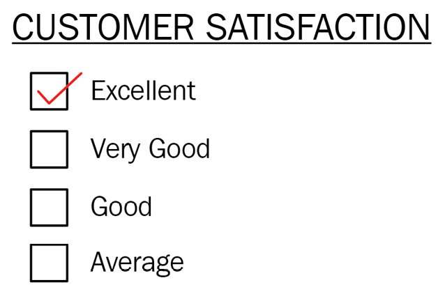
Figure 1.6 – A survey study example

Figure 1.6 – A survey study example

The previous example is one of two types of non-probability sampling methods that we want to discuss here. This method is convenience sampling. In convenience sampling, researchers choose members the most accessible to the researchers from a population to form a sample. This method is easy and inexpensive but generalizing the results obtained to the whole population is questionable.

Quota sampling is another type of non-probability sampling where a sample group is selected to be representative of a larger population in a non-random way. For example, recruiters with limited time can use the quota sampling method to search for potential candidates from professional social networks (LinkedIn, Indeed.com, etc.) and interview them. This method is cost-effective and saves time but presents bias during the selection process.

In this section, we provided an overview of probability and non-probability sampling. Each strategy has advantages and disadvantages, but they help us to minimize risks, such as bias. A well-planned sampling strategy will also help reduce errors in predictive modeling.

Summary

In this chapter, we discussed installing and setting up the Python environment to run the Statsmodels API and other requisite open-source packages. We also discussed populations versus samples and the requirements to gain inference from samples. Finally, we explained several different common sampling methods used in statistical and machine learning models.

In the next chapter, we will begin a discussion on statistical distributions and their implications for building statistical models. In Chapter 3, Hypothesis Testing, we will begin discussing hypothesis testing in depth, expanding on the concepts discussed in the Observational study section of this chapter. We will also discuss power analysis, which is a useful tool for determining the sample size based on existing sample data parameters and the desired levels of statistical significance.

Left arrow icon Right arrow icon
Download code icon Download Code

Key benefits

  • Gain expertise in identifying and modeling patterns that generate success
  • Explore the concepts with Python using important libraries such as stats models
  • Learn how to build models on real-world data sets and find solutions to practical challenges

Description

The ability to proficiently perform statistical modeling is a fundamental skill for data scientists and essential for businesses reliant on data insights. Building Statistical Models with Python is a comprehensive guide that will empower you to leverage mathematical and statistical principles in data assessment, understanding, and inference generation. This book not only equips you with skills to navigate the complexities of statistical modeling, but also provides practical guidance for immediate implementation through illustrative examples. Through emphasis on application and code examples, you’ll understand the concepts while gaining hands-on experience. With the help of Python and its essential libraries, you’ll explore key statistical models, including hypothesis testing, regression, time series analysis, classification, and more. By the end of this book, you’ll gain fluency in statistical modeling while harnessing the full potential of Python's rich ecosystem for data analysis.

Who is this book for?

If you are looking to get started with building statistical models for your data sets, this book is for you! Building Statistical Models in Python bridges the gap between statistical theory and practical application of Python. Since you’ll take a comprehensive journey through theory and application, no previous knowledge of statistics is required, but some experience with Python will be useful.

What you will learn

  • Explore the use of statistics to make decisions under uncertainty
  • Answer questions about data using hypothesis tests
  • Understand the difference between regression and classification models
  • Build models with stats models in Python
  • Analyze time series data and provide forecasts
  • Discover Survival Analysis and the problems it can solve
Estimated delivery fee Deliver to Lithuania

Premium delivery 7 - 10 business days

€25.95
(Includes tracking information)

Product Details

Country selected
Publication date, Length, Edition, Language, ISBN-13
Publication date : Aug 31, 2023
Length: 420 pages
Edition : 1st
Language : English
ISBN-13 : 9781804614280
Category :
Languages :
Concepts :

What do you get with Print?

Product feature icon Instant access to your digital eBook copy whilst your Print order is Shipped
Product feature icon Colour book shipped to your preferred address
Product feature icon Download this book in EPUB and PDF formats
Product feature icon Access this title in our online reader with advanced features
Product feature icon DRM FREE - Read whenever, wherever and however you want
Product feature icon AI Assistant (beta) to help accelerate your learning
OR
Modal Close icon
Payment Processing...
tick Completed

Shipping Address

Billing Address

Shipping Methods
Estimated delivery fee Deliver to Lithuania

Premium delivery 7 - 10 business days

€25.95
(Includes tracking information)

Product Details

Publication date : Aug 31, 2023
Length: 420 pages
Edition : 1st
Language : English
ISBN-13 : 9781804614280
Category :
Languages :
Concepts :

Packt Subscriptions

See our plans and pricing
Modal Close icon
€18.99 billed monthly
Feature tick icon Unlimited access to Packt's library of 7,000+ practical books and videos
Feature tick icon Constantly refreshed with 50+ new titles a month
Feature tick icon Exclusive Early access to books as they're written
Feature tick icon Solve problems while you work with advanced search and reference features
Feature tick icon Offline reading on the mobile app
Feature tick icon Simple pricing, no contract
€189.99 billed annually
Feature tick icon Unlimited access to Packt's library of 7,000+ practical books and videos
Feature tick icon Constantly refreshed with 50+ new titles a month
Feature tick icon Exclusive Early access to books as they're written
Feature tick icon Solve problems while you work with advanced search and reference features
Feature tick icon Offline reading on the mobile app
Feature tick icon Choose a DRM-free eBook or Video every month to keep
Feature tick icon PLUS own as many other DRM-free eBooks or Videos as you like for just €5 each
Feature tick icon Exclusive print discounts
€264.99 billed in 18 months
Feature tick icon Unlimited access to Packt's library of 7,000+ practical books and videos
Feature tick icon Constantly refreshed with 50+ new titles a month
Feature tick icon Exclusive Early access to books as they're written
Feature tick icon Solve problems while you work with advanced search and reference features
Feature tick icon Offline reading on the mobile app
Feature tick icon Choose a DRM-free eBook or Video every month to keep
Feature tick icon PLUS own as many other DRM-free eBooks or Videos as you like for just €5 each
Feature tick icon Exclusive print discounts

Frequently bought together


Stars icon
Total 113.97
Building Statistical Models in Python
€37.99
Machine Learning Engineering  with Python
€37.99
Exploratory Data Analysis with Python Cookbook
€37.99
Total 113.97 Stars icon
Banner background image

Table of Contents

21 Chapters
Part 1:Introduction to Statistics Chevron down icon Chevron up icon
Chapter 1: Sampling and Generalization Chevron down icon Chevron up icon
Chapter 2: Distributions of Data Chevron down icon Chevron up icon
Chapter 3: Hypothesis Testing Chevron down icon Chevron up icon
Chapter 4: Parametric Tests Chevron down icon Chevron up icon
Chapter 5: Non-Parametric Tests Chevron down icon Chevron up icon
Part 2:Regression Models Chevron down icon Chevron up icon
Chapter 6: Simple Linear Regression Chevron down icon Chevron up icon
Chapter 7: Multiple Linear Regression Chevron down icon Chevron up icon
Part 3:Classification Models Chevron down icon Chevron up icon
Chapter 8: Discrete Models Chevron down icon Chevron up icon
Chapter 9: Discriminant Analysis Chevron down icon Chevron up icon
Part 4:Time Series Models Chevron down icon Chevron up icon
Chapter 10: Introduction to Time Series Chevron down icon Chevron up icon
Chapter 11: ARIMA Models Chevron down icon Chevron up icon
Chapter 12: Multivariate Time Series Chevron down icon Chevron up icon
Part 5:Survival Analysis Chevron down icon Chevron up icon
Chapter 13: Time-to-Event Variables – An Introduction Chevron down icon Chevron up icon
Chapter 14: Survival Models Chevron down icon Chevron up icon
Index Chevron down icon Chevron up icon
Other Books You May Enjoy Chevron down icon Chevron up icon

Customer reviews

Top Reviews
Rating distribution
Full star icon Full star icon Full star icon Full star icon Half star icon 4.9
(11 Ratings)
5 star 90.9%
4 star 9.1%
3 star 0%
2 star 0%
1 star 0%
Filter icon Filter
Top Reviews

Filter reviews by


Dror Oct 01, 2023
Full star icon Full star icon Full star icon Full star icon Full star icon 5
Statistics is a fundamental discipline concerned with the collection, organization, analysis, interpretation, and presentation of data. While Python—an extremely popular general-purpose programming language—has become the programming language of choice for computation in most science and engineering disciplines, most (software-oriented) statistics books still teach statistics using the more special-purpose R language.This unique and highly practical book provides a gentle introduction to statistics and to using the Python programming language for building statistical models. It begins with a clear and useful introduction to statistics, including sampling, data distributions, hypothesis testing, and parametric and non-parametric statistical tests. It then progresses to describe in detail how to build statistical models using Python for a variety of problems, including for regression, classification, time-series, and survival analysis. The descriptions are clear and concise, and gradually present additional common and helpful Python packages for performing statistical analysis. The accompanying GitHub repository includes practical and detailed code examples, and is very helpful in reinforcing the materials and concepts presented in the book.I highly recommend this book to anyone interested in learning statistics and how to use Python for building statistical models. It requires no more than basic knowledge of the Python programming language, and will be ideal for data scientists, analysts, and industry professionals who are taking their first steps in the world of statistics or want to expand their knowledge in this area.Highly recommended!
Amazon Verified review Amazon
JRVV Oct 19, 2023
Full star icon Full star icon Full star icon Full star icon Full star icon 5
The book provides a broad primer on statistical modeling using Python. This book can also serve as a starting point to those who eventually want to go into machine learning. Recommended.
Amazon Verified review Amazon
Amazon Customer Oct 02, 2023
Full star icon Full star icon Full star icon Full star icon Full star icon 5
This book is exceptionally crafted, serving as a comprehensive review of fundamental statistical knowledge, complemented with practical Python codes. Unlike other market options, which either focus solely on theory or coding, lacking depth in theoretical insight, this book seamlessly bridges theory to application. While many statistical texts predominantly utilize the R language, this book's emphasis on Python is a refreshing change. It not only rejuvenates and reinforces my existing knowledge but also significantly advances my understanding of Statistics and Machine Learning. It stands out as a balanced and insightful resource for both theoretical comprehension and practical application in the field.
Amazon Verified review Amazon
Steven Fernandes Oct 09, 2023
Full star icon Full star icon Full star icon Full star icon Full star icon 5
The authors offer a compelling dive into making informed decisions under uncertainty, equipping readers with practical skills, such as hypothesis testing and data analysis. They thoughtfully elucidate the distinctions between regression and classification models and provide a hands-on approach to building models using Python's statsmodels. The text also insightfully explores time-series data analysis, forecasting, and survival analysis, adeptly linking theory with real-world applications. This book emerges as an invaluable guide for both beginners and seasoned practitioners, intertwining robust theoretical constructs with practical applicability in data analysis and model-building, rendering it a must-read in the field of data science.
Amazon Verified review Amazon
Ratan Nov 23, 2023
Full star icon Full star icon Full star icon Full star icon Full star icon 5
Authors have done a good job in maintaining the comprehensiveness of the book. They have maintained adequate amount of mathematics what is needed. I particularly loved the way they have presented Hypothesis testing for models which is often missing in many places. They have nicely covered both parametric and non parametric testing.The other part I liked was somewhat less visited topic survival analysis. Overall I found this book an excellent read ! Definitely recommend it.
Amazon Verified review Amazon
Get free access to Packt library with over 7500+ books and video courses for 7 days!
Start Free Trial

FAQs

What is the delivery time and cost of print book? Chevron down icon Chevron up icon

Shipping Details

USA:

'

Economy: Delivery to most addresses in the US within 10-15 business days

Premium: Trackable Delivery to most addresses in the US within 3-8 business days

UK:

Economy: Delivery to most addresses in the U.K. within 7-9 business days.
Shipments are not trackable

Premium: Trackable delivery to most addresses in the U.K. within 3-4 business days!
Add one extra business day for deliveries to Northern Ireland and Scottish Highlands and islands

EU:

Premium: Trackable delivery to most EU destinations within 4-9 business days.

Australia:

Economy: Can deliver to P. O. Boxes and private residences.
Trackable service with delivery to addresses in Australia only.
Delivery time ranges from 7-9 business days for VIC and 8-10 business days for Interstate metro
Delivery time is up to 15 business days for remote areas of WA, NT & QLD.

Premium: Delivery to addresses in Australia only
Trackable delivery to most P. O. Boxes and private residences in Australia within 4-5 days based on the distance to a destination following dispatch.

India:

Premium: Delivery to most Indian addresses within 5-6 business days

Rest of the World:

Premium: Countries in the American continent: Trackable delivery to most countries within 4-7 business days

Asia:

Premium: Delivery to most Asian addresses within 5-9 business days

Disclaimer:
All orders received before 5 PM U.K time would start printing from the next business day. So the estimated delivery times start from the next day as well. Orders received after 5 PM U.K time (in our internal systems) on a business day or anytime on the weekend will begin printing the second to next business day. For example, an order placed at 11 AM today will begin printing tomorrow, whereas an order placed at 9 PM tonight will begin printing the day after tomorrow.


Unfortunately, due to several restrictions, we are unable to ship to the following countries:

  1. Afghanistan
  2. American Samoa
  3. Belarus
  4. Brunei Darussalam
  5. Central African Republic
  6. The Democratic Republic of Congo
  7. Eritrea
  8. Guinea-bissau
  9. Iran
  10. Lebanon
  11. Libiya Arab Jamahriya
  12. Somalia
  13. Sudan
  14. Russian Federation
  15. Syrian Arab Republic
  16. Ukraine
  17. Venezuela
What is custom duty/charge? Chevron down icon Chevron up icon

Customs duty are charges levied on goods when they cross international borders. It is a tax that is imposed on imported goods. These duties are charged by special authorities and bodies created by local governments and are meant to protect local industries, economies, and businesses.

Do I have to pay customs charges for the print book order? Chevron down icon Chevron up icon

The orders shipped to the countries that are listed under EU27 will not bear custom charges. They are paid by Packt as part of the order.

List of EU27 countries: www.gov.uk/eu-eea:

A custom duty or localized taxes may be applicable on the shipment and would be charged by the recipient country outside of the EU27 which should be paid by the customer and these duties are not included in the shipping charges been charged on the order.

How do I know my custom duty charges? Chevron down icon Chevron up icon

The amount of duty payable varies greatly depending on the imported goods, the country of origin and several other factors like the total invoice amount or dimensions like weight, and other such criteria applicable in your country.

For example:

  • If you live in Mexico, and the declared value of your ordered items is over $ 50, for you to receive a package, you will have to pay additional import tax of 19% which will be $ 9.50 to the courier service.
  • Whereas if you live in Turkey, and the declared value of your ordered items is over € 22, for you to receive a package, you will have to pay additional import tax of 18% which will be € 3.96 to the courier service.
How can I cancel my order? Chevron down icon Chevron up icon

Cancellation Policy for Published Printed Books:

You can cancel any order within 1 hour of placing the order. Simply contact customercare@packt.com with your order details or payment transaction id. If your order has already started the shipment process, we will do our best to stop it. However, if it is already on the way to you then when you receive it, you can contact us at customercare@packt.com using the returns and refund process.

Please understand that Packt Publishing cannot provide refunds or cancel any order except for the cases described in our Return Policy (i.e. Packt Publishing agrees to replace your printed book because it arrives damaged or material defect in book), Packt Publishing will not accept returns.

What is your returns and refunds policy? Chevron down icon Chevron up icon

Return Policy:

We want you to be happy with your purchase from Packtpub.com. We will not hassle you with returning print books to us. If the print book you receive from us is incorrect, damaged, doesn't work or is unacceptably late, please contact Customer Relations Team on customercare@packt.com with the order number and issue details as explained below:

  1. If you ordered (eBook, Video or Print Book) incorrectly or accidentally, please contact Customer Relations Team on customercare@packt.com within one hour of placing the order and we will replace/refund you the item cost.
  2. Sadly, if your eBook or Video file is faulty or a fault occurs during the eBook or Video being made available to you, i.e. during download then you should contact Customer Relations Team within 14 days of purchase on customercare@packt.com who will be able to resolve this issue for you.
  3. You will have a choice of replacement or refund of the problem items.(damaged, defective or incorrect)
  4. Once Customer Care Team confirms that you will be refunded, you should receive the refund within 10 to 12 working days.
  5. If you are only requesting a refund of one book from a multiple order, then we will refund you the appropriate single item.
  6. Where the items were shipped under a free shipping offer, there will be no shipping costs to refund.

On the off chance your printed book arrives damaged, with book material defect, contact our Customer Relation Team on customercare@packt.com within 14 days of receipt of the book with appropriate evidence of damage and we will work with you to secure a replacement copy, if necessary. Please note that each printed book you order from us is individually made by Packt's professional book-printing partner which is on a print-on-demand basis.

What tax is charged? Chevron down icon Chevron up icon

Currently, no tax is charged on the purchase of any print book (subject to change based on the laws and regulations). A localized VAT fee is charged only to our European and UK customers on eBooks, Video and subscriptions that they buy. GST is charged to Indian customers for eBooks and video purchases.

What payment methods can I use? Chevron down icon Chevron up icon

You can pay with the following card types:

  1. Visa Debit
  2. Visa Credit
  3. MasterCard
  4. PayPal
What is the delivery time and cost of print books? Chevron down icon Chevron up icon

Shipping Details

USA:

'

Economy: Delivery to most addresses in the US within 10-15 business days

Premium: Trackable Delivery to most addresses in the US within 3-8 business days

UK:

Economy: Delivery to most addresses in the U.K. within 7-9 business days.
Shipments are not trackable

Premium: Trackable delivery to most addresses in the U.K. within 3-4 business days!
Add one extra business day for deliveries to Northern Ireland and Scottish Highlands and islands

EU:

Premium: Trackable delivery to most EU destinations within 4-9 business days.

Australia:

Economy: Can deliver to P. O. Boxes and private residences.
Trackable service with delivery to addresses in Australia only.
Delivery time ranges from 7-9 business days for VIC and 8-10 business days for Interstate metro
Delivery time is up to 15 business days for remote areas of WA, NT & QLD.

Premium: Delivery to addresses in Australia only
Trackable delivery to most P. O. Boxes and private residences in Australia within 4-5 days based on the distance to a destination following dispatch.

India:

Premium: Delivery to most Indian addresses within 5-6 business days

Rest of the World:

Premium: Countries in the American continent: Trackable delivery to most countries within 4-7 business days

Asia:

Premium: Delivery to most Asian addresses within 5-9 business days

Disclaimer:
All orders received before 5 PM U.K time would start printing from the next business day. So the estimated delivery times start from the next day as well. Orders received after 5 PM U.K time (in our internal systems) on a business day or anytime on the weekend will begin printing the second to next business day. For example, an order placed at 11 AM today will begin printing tomorrow, whereas an order placed at 9 PM tonight will begin printing the day after tomorrow.


Unfortunately, due to several restrictions, we are unable to ship to the following countries:

  1. Afghanistan
  2. American Samoa
  3. Belarus
  4. Brunei Darussalam
  5. Central African Republic
  6. The Democratic Republic of Congo
  7. Eritrea
  8. Guinea-bissau
  9. Iran
  10. Lebanon
  11. Libiya Arab Jamahriya
  12. Somalia
  13. Sudan
  14. Russian Federation
  15. Syrian Arab Republic
  16. Ukraine
  17. Venezuela