AI techniques for video games
In this section, we will look at some of the AI techniques that are commonly used in different types of games. We'll learn how to implement each of these features in Unity in the upcoming chapters. Since this book does not focus on AI techniques themselves but on implementing these techniques inside Unity, we won't look at them in too much detail here. So, let's just take this as a crash course before diving into the implementation details.
If you want to learn more about AI for games, there are some great books, such as Programming Game AI by Example, by Mat Buckland, and Artificial Intelligence for Games, by Ian Millington and John Funge. In addition, the AI Game Programming Wisdom and Game AI Pro series also contain a lot of valuable resources and articles on the latest AI techniques.
Finite state machines
Finite State Machines (FSMs) are probably one of the simplest, most used, and most discussed AI models and, for most games, they represent the only AI technique. A state machine consists of a finite number of states that are connected by one or more transitions, resulting in a data structure known as a graph. Each game entity starts with an initial state. Then, environment events trigger specific rules that will make the entity move into another state. Such triggering rules are called transitions. A game entity can only be in one state at any given time.
For example, let's consider an AI guard character in a typical shooting game. Its states could be as simple as patrolling, chasing, and shooting:
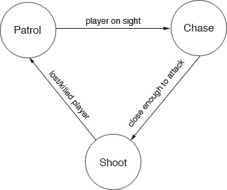
Figure 1.1 – A simple FSM for an AI guard character
There are four components in a simple FSM:
- States: This component defines a set of states that a game entity or an NPC can choose from (Patrol, Chase, and Shoot).
- Transitions: This component defines the relationships between different states.
- Rules: This component defines when to perform a state transition (Player in sight, Close enough to attack, and Lost/killed player).
- Events: This is the component that will trigger to check the rules (the guard's visible area, distance to the player, and so on).
So, a monster in Quake 2 may have the following states: standing, walking, running, dodging, attacking, idle, and searching.
FSMs are widely used in games because they are simple to implement using only a bunch of if or switch statements, but they are still powerful enough for simple and somewhat complex games. On the other hand, they can get messy when we need a lot of states and transitions. We'll learn how to manage a simple FSM in the next chapter.
Randomness and probability in AI
Imagine an enemy bot in a First-Person Shooter (FPS) game that can always kill the player with a headshot or an opponent in a racing game who always chooses the best route and never collides with any obstacle. Such a level of intelligence will make the game so hard that it will become almost impossible to win and, as a consequence, it will be frustrating to play. On the opposite side of the spectrum, imagine an enemy that chooses the same predictable route whenever it tries to escape from the player. After a couple of games, the player will learn the enemy's pattern, and the game will feel boring. AI-controlled entities that behave the same way every time the player encounters them make the game predictable, easy to win, and therefore dull.
Of course, there are some cases in which intentional predictability is a desired feature. In stealth games, for instance, we want the players to be able to predict the path of the enemies so that the players can plan a sneaking route. But in other cases, unintentional predictability can interfere with the game's engagement and make the player feel like the game is not challenging or fair enough. One way to fix these too-perfect or too-stupid AIs is to introduce intentional mistakes in their behavior. In games, we introduce randomness and probability in the decision-making process of AI calculations.
There are multiple scenarios where we may want to introduce a bit of randomness. The most straightforward case is when the NPC has no information and/or it doesn't matter what decision it makes. For instance, in a shooting game, an enemy under fire may want to decide where to cover. So, instead of always moving it to the closest cover, we may wish to instruct the NPCs to sometimes choose a slightly far-away cover.
In other cases, we can use randomness for the outcomes of a decision. For example, we can use randomness for hit probabilities, add or subtract random bits of damage to/from base damage, or make an NPC hesitate before they start shooting.
The sensor system
Our AI characters need to know their surroundings and the world they interact with to make a particular decision. Such information includes the following:
- The position of the player: This is used to decide whether to attack or chase or keep patrolling.
- Buildings and nearby objects: This is used to hide or take cover.
- The player's health and the AI's health: This is used to decide whether to retreat or advance.
- Location of resources on the map in a Real-Time Strategy (RTS) game: This is used to occupy and collect resources that are required to update and/or produce other units.
As you can imagine, choosing the correct method to collect game information can vary a lot, depending on the type of game we are trying to build. In the next few sections, we'll look at two basic strategies: polling and message (event) systems.
Polling
One method to collect such information is polling. Polling consists of directly checking for the preceding information in Unity's FixedUpdate method of our AI character. In this way, AI characters can just poll the information they are interested in from the game world, do the checks, and take action accordingly. Polling works great if there aren't too many things to check.
To make this method more efficient, we may want to program the characters to poll the world states at different rates so that we do not have all the characters checking everything at once. For instance, we may divide the polling agents into 10 groups (G1, G2, G3, and so on) and assign the polling for each group at different frames (for example, G1 will poll at frame 0, 60, 120, and so on; G2 will poll at frame 10, 70, 130, and so on).
As another example, we may decide to change the polling frequency based on the enemy's type or state. For instance, enemies that are disengaged and far away may poll every 3-4 seconds, while enemies closer to the player and under attack may want to poll every 0.5 seconds.
However, polling is no longer enough as soon as the game gets bigger. Therefore, in more massive games with more complex AI systems, we need to implement an event-driven method using a global messaging system.
Messaging systems
In a messaging system, the game communicates events between the AI entity and the player, the world, or the other AI entities through asynchronous messages. For example, when the player attacks an enemy unit inside a group of patrol guards, the other AI units need to know about this incident so that they can start searching for and attacking the player.
If we were using the polling method, our AI entities would need to check the state of all of the other AI entities to find out if one of them has been attacked. However, we can implement this in a more manageable and scalable fashion: we can register the AI characters that are interested in a particular event as listeners of that event; then, if that event occurs, our messaging system will broadcast this information to all listeners. The AI entities can then take the appropriate actions or perform further checks.
This event-driven system does not necessarily provide a faster mechanism than polling. Still, it provides a convenient, central checking system that senses the world and informs the interested AI agents, rather than having each agent check the same event in every frame. In reality, both polling and messaging systems are used together most of the time. For example, the AI may poll for more detailed information when it receives an event from the messaging system.
Flocking, swarming, and herding
Many living beings such as birds, fish, insects, and land animals perform specific operations such as moving, hunting, and foraging in groups. They stay and hunt in groups because it makes them stronger and safer from predators than pursuing goals individually. So, let's say you want a group of birds flocking, swarming around in the sky; it'll cost too much time and effort for animators to design the movement and animations of each bird. However, if we apply some simple rules for each bird to follow, we can achieve an emergent intelligence for the whole group with complex, global behavior.
One pioneer of this concept is Craig Reynolds, who presented such a flocking algorithm in his 1987 SIGGRAPH paper, Flocks, Herds, and Schools – A Distributed Behavioral Model. He coined the term boid, which sounds like "bird" but refers to a bird-like object. He proposed three simple rules to apply to each unit:
- Separation: Each boid needs to maintain a minimum distance from neighboring boids to avoid hitting them (short-range repulsion).
- Alignment: Each boid needs to align itself with the average direction of its neighbors and then move in the same velocity with them as a flock.
- Cohesion: Each boid is attracted to the group's center of mass (long-range attraction).
These three simple rules are all we need to implement a realistic and reasonably complex flocking behavior for birds. This doesn't only work with birds. Flocking behaviors are useful for modeling a crowd or even a couple of NPCs that will follow the player during the game.
We'll learn how to implement such a flocking system in Unity in Chapter 5, Flocking.
Path following and steering
Sometimes, we want our AI characters to roam the game world and follow a roughly guided or thoroughly defined path. For example, in a racing game, the AI opponents need to navigate a road. In that case, simple reactive algorithms, such as our flocking boid algorithm, are not powerful enough to solve this problem. Still, in the end, it all comes down to dealing with actual movements and steering behaviors. Steering behaviors for AI characters has been a research topic for a couple of decades now.
One notable paper in this field is Steering Behaviors for Autonomous Characters, again by Craig Reynolds, presented in 1999 at the Game Developers Conference (GDC). He categorized steering behaviors into the following three layers:

Figure 1.2 – Hierarchy of motion behaviors
To understand these layers, let's look at an example. Imagine that you are working at your desk on a hot summer afternoon. You are thirsty, and you want a cold glass of iced tea. So, we start from the first layer: we want a cold glass of iced tea (setting the goal), and we plan out what we need to do to get it. We probably need to go to the kitchen (unless you have a mini-fridge under your desk), fetch an empty glass, and then move to the fridge, open it, and get the iced tea (we have made a high-level plan).
Now, we move to the second layer. Unless your kitchen is a direct straight line from your desk, you need to determine a path: go around the desk, move through a corridor, navigate around the kitchen furniture until you reach the cabinet with the glasses, and so on. Now that you have a path, it is time to move to the third layer: walking the path. In this example, the third layer is represented by your body, skeleton, and muscles moving you along the path.
Information
Don't worry – you don't need to master all three layers. As an AI programmer, you only need to focus on the first two. The third layer is usually handled by graphic programmers – in particular, animators.
After describing these three layers, Craig Reynolds explains how to design and implement standard steering behaviors for individual AI characters. Such behaviors include seek and flee, pursue and evade, wander, arrival, obstacle avoidance, wall following, and path following.
We'll implement some of these behaviors in Unity in Chapter 6, Path Following and Steering Behaviors.
A* pathfinding
There are many games where you can find monsters or enemies that follow the player or move to a particular point while avoiding obstacles. For example, let's take a look at a typical RTS game. You can select a group of units and click a location where you want them to move or click on the enemy units to attack them.
Then, your units need to find a way to reach the goal without colliding with the obstacles. Of course, the enemy units also need to be able to do the same. The barriers could be different for different units. For example, an airforce unit may pass over a mountain, while the ground or artillery units need to find a way around it.
A* (pronounced A-star) is a pathfinding algorithm that's widely used in games because of its performance, accuracy, and ease of implementation. Let's look at an example to see how it works. Let's say we want our unit to move from point A to point B, but there's a wall in the way, and it can't go straight toward the target. So, it needs to find a way to point B while avoiding the wall:

Figure 1.3 – Top-down view of our map
This is a simple 2D example, but we can apply the same idea to 3D environments. To find the path from point A to point B, we need to know more about the map, such as the position of obstacles. For that, we can split our whole map into small tiles that represent the entire map in a grid format, as shown in the following diagram:

Figure 1.4 – Map represented in a 2D grid
The tiles can also be of other shapes, such as hexagons or triangles. Each shape comes with its advantages. For instance, hexagonal tiles are convenient because they do not have the problem of diagonal moves (all the hexagons surrounding a target hexagon are at the same distance). In this example, though, we have used square tiles because they are the more intuitive shape that comes to mind when we think about grids.
Now, we can reference our map in a small 2D array.
We can represent our map with a 5x5 grid of square tiles for a total of 25 tiles. Now, we can start searching for the best path to reach the target. How do we do this? By calculating the movement score of each tile that's adjacent to the starting tile that is not occupied by an obstacle, and then choosing the tile with the lowest cost.
If we don't consider the diagonal movements, there are four possible adjacent tiles to the player. Now, we need to use two numbers to calculate the movement score for each of those tiles. Let's call them G and H, where G is the cost to move from the starting tile to the current tile, and H is the estimated cost to reach the target tile from the current tile.
Let's call F the sum of G and H, (F = G + H) – that is, the final score of that tile:
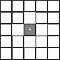
Figure 1.5 – Valid adjacent tiles
In our example, to estimate H, we'll use a simple method called Manhattan length (also known as taxicab geometry). According to this method, the distance (cost) between A and B is the number of horizontal tiles, A and B, plus the number of vertical tiles between A and B:
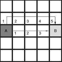
Figure 1.6 – Calculating G
The G value, on the other hand, represents the cost so far during the search. The preceding diagram shows the calculations of G with two different paths. To compute the current G, we must add 1 (the cost of moving one tile) to the previous tile's G score. However, we can give different costs to different tiles. For example, we may want to set a higher movement cost for diagonal movements (if we are considering them) or, for instance, to tiles occupied by a pond or a muddy road.
Now that we know how to get G, let's learn how to calculate H. The following diagram shows the H value for different starting tiles. Even in this case, we use the Manhattan distance:

Figure 1.7 – Calculating H
So, now that we know how to get G and H, let's go back to our original example to figure out the shortest path from A to B. First, we must choose the starting tile and collect all its adjacent tiles, as shown in the following diagram. Then, we must calculate each tile's G and H scores, as shown in the tile's lower left and right corners. Finally, we must get the final score, F, by adding G and H together. You can see the F score in the tile's top-left corner.
Now, we must choose the tile with the lowest F score as our next tile and store the previous tile as its parent. Note that keeping records of each tile's parents is crucial because we will use this backlink later to trace the sequence of nodes from the end to the start to obtain the final path. In this example, we must choose the tile to the right of the starting position and consider it the current tile:

Figure 1.8 – Starting position
From the current tile, we repeat this process, starting with collecting the valid adjacent tiles. There are only two free adjacent tiles this time: the one above the current tile and the one at the bottom (in fact, the left tile is the starting tile – which we've already examined – and the obstacle occupies the right tile). We calculate G and H, and then the F score of those new adjacent tiles.
This time, we have four tiles on our map, all with the same score: six. Therefore, we can choose any of them. In fact, in the end, we will find the shortest path independently of which tile we explore first (proving the math behind this statement is outside the scope of this book):
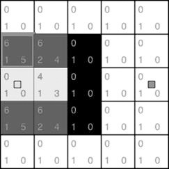
Figure 1.9 – Second step
In this example, from the group of tiles with a cost of 6, we chose the tile at the top left as the starting position. Again, we must examine the adjacent tiles. In this step, there's only one new adjacent tile with a calculated F score of 8. Because the lowest score is still 6 right now, we can choose any tile with a score of 6:
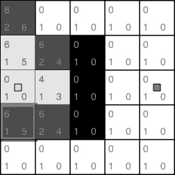
Figure 1.10 – Third step
If we repeat this process until we reach our target tile, we'll end up with a board that shows all the scores for each free tile:
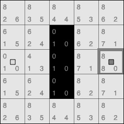
Figure 1.11 – Reach target
There is only one step left. Do you remember the parent links that we stored in each node? Now, starting from the target tile, we must use the stored parent tile to trace back a list of tiles. The resulting list will be a path that looks something like this:
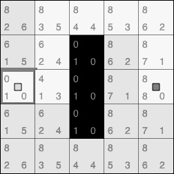
Figure 1.12 – Path traced back
What we explained here is the essence of the A* pathfinding algorithm, which is the basic founding block of any pathfinding algorithm. Fortunately, since Unity 3.5, a couple of new features such as automatic navigation mesh generation and the NavMesh Agent make implementing pathfinding in your games much more accessible. As a result, you may not even need to know anything about A* to implement pathfinding for your AI characters. Nonetheless, knowing how the system works behind the scenes is essential to becoming a solid AI programmer.
We'll talk about NavMesh in the next section and then in more detail in Chapter 8, Navigation Mesh.
Navigation meshes
Now that you know the basics of the A* pathfinding algorithm, you may notice that using a grid in A* requires many steps to get the shortest path between the start and target position. It may not seem notable but searching for a path tile-by-tile for huge maps with thousands of mostly empty tiles is a severe waste of computational power. So, games often use waypoints as a guide to move the AI characters as a simple and effective way to use fewer computation resources.
Let's say we want to move our AI character from point A to point B, and we've set up three waypoints, as shown in the following diagram:

Figure 1.13 – Waypoints
All we have to do now is apply the A* algorithm to the waypoints (there are fewer of these compared to the number of tiles) and then simply move the character in a straight line from waypoint to waypoint.
However, waypoints are not without issues. What if we want to update the obstacles in our map? We'll have to place the waypoints again for the updated map, as shown in the following diagram:
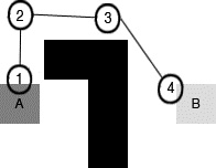
Figure 1.14 – New waypoints
Moreover, following each node to the target produces characters that look unrealistic. For instance, they move in straight lines, followed by an abrupt change of direction, much like the mechanical puppets in a theme park's attraction. Or the path that connects two waypoints may be too close to the obstacles. For example, look at the preceding diagrams; the AI character will likely collide with the wall where the path is close to the wall.
If that happens, our AI will keep trying to go through the wall to reach the next target, but it won't be able to, and it will get stuck there. Sure, we could make the path more realistic by smoothing out the zigzag path using splines, or we could manually check each path to avoid grazing the edges of obstacles. However, the problem is that the waypoints don't contain any information about the environment other than the trajectory that's connecting two nodes.
To address such situations, we're going to need a tremendous number of waypoints, which are very hard to manage. So, for everything other than straightforward games, we must exchange the computational cost of a grid with the mental and design cost of managing hundreds of waypoints.
Fortunately, there is a better solution: using a navigation mesh. A navigation mesh (often called NavMesh) is another graph structure that we can use to represent our world, similar to square tile-based grids and waypoint graphs:
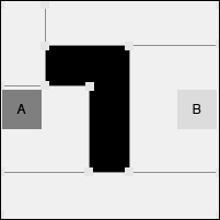
Figure 1.15 – Navigation mesh
A NavMesh uses convex polygons to represent the areas in the map where an AI entity can travel. The most crucial benefit of using a NavMesh is that it contains much more information about the environment than a waypoint system. With a NavMesh, we can automatically adjust our path safely because we know that our AI entities can move freely inside a region. Another advantage of using a NavMesh is that we can use the same mesh for different types of AI entities. Different AI entities can have different properties such as size, speed, and movement abilities. For instance, a set of waypoints may be suitable for human characters, but they may not work nicely for flying creatures or AI-controlled vehicles. Those may need different sets of waypoints (with all the problems that this adds).
However, programmatically generating a NavMesh based on a scene is a somewhat complicated process. Fortunately, Unity includes a built-in NavMesh generator.
Since this is not a book on core AI techniques, we won't go into how to generate such NavMeshes. Instead, we'll learn how to efficiently use Unity's NavMesh to implement pathfinding for our AI characters.
Behavior trees
Behavior trees are another technique that's used to represent and control the logic behind AI characters' decisions. They have become popular for their applications in AAA games such as Halo and Spore. We briefly covered FSMs earlier in this chapter, which is a straightforward way to define the logic of AI characters based on the transition between different states in reaction to game events. However, FSMs have two main issues: they are challenging to scale and reuse.
To support all the scenarios where we want our characters to be, we need to add a lot of states and hardwire many transitions. So, we need something that scales better with more extensive problems. Behavior trees represent a sensible step in the right direction.
As its name suggests, the essence of a behavior tree is a tree-like data structure. The leaves of such trees are called tasks, and they represent our character's actions (for instance, attack, chase, patrol, hide, and so on) or sensory input (for example, Is the player near? or Am I close enough to attack?). Instead, the internal nodes of the trees are represented by control flow nodes, which guide the execution of the tree. Sequence, Selector, and Parallel Decorator are commonly used control flow nodes.
Now, let's try to reimplement the example from the Finite state machines section using a behavior tree. First, we can break all the transitions and states into basic tasks:

Figure 1.16 – Tasks
Now, let's look at a Selector node. We represent a Selector with a circle with a question mark inside it. When executed, a Selector node tries to execute all the child tasks/sub-trees in sequential order until the first one that returns with success. In other words, if we have a Selector with four children (for example, A, B, C, and D), the Selector node executes A first. If A fails, then the Selector executes B. If B fails, then it executes C, and so on. If any of the tasks return a Success, then the Sequence returns a Success as soon as that task completes.
In the following example, the Selector node first chooses to attack the player. If the Attack task returns a Success (that is, if the player is in attack range), the Selector node stops the execution and returns with a Success to its parent node – if there is one. Instead, if the Attack task returns with a failure, the Selector node moves to the Chase task. Here, we repeat what we did previously: if the Chase task succeeds, the Selector node succeeds; if the Chase task fails, it tries the Patrol task, and so on:
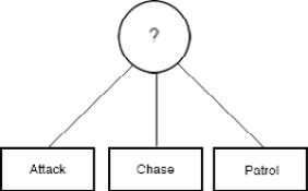
Figure 1.17 – Selector node
What about the other kind of tasks – the ones that check the game state? We use them with Sequence nodes, which are usually represented with a rectangle with an arrow inside them. A Sequence node is similar to a Selector node with a crucial difference: it only returns a Success message if every sub-tree returns with a Success. In other words, if we have a Sequence with four children (for example, A, B, C, and D), the Sequence node will execute A, then B, then C, and finally D. If all the tasks return a Success, then the Sequence returns a Success.
In the following example, the first Sequence node checks whether the player character is close enough to attack. If this task succeeds, it will proceed to the next task: attacking the player. If the Attack task also returns with a Success message, the whole Sequence terminates with success. Instead, if the Close Enough to Attack? task fails, then the Sequence node does not proceed to the Attack task and returns a failed status to the parent Selector node. Then, the Selector chooses the next task in the Sequence, Lost or Killed Player, and the execution continues:

Figure 1.18 – Sequence tasks
The other two common nodes are Parallel and Decorator. A Parallel node executes all of its child tasks simultaneously (while the Sequence and Selector nodes only execute their child trees one by one). A Decorator is another type of node that has only one child. It is used to change the behavior of its own single child's sub-tree, for instance, to run it multiple times or invert the subtree's result (if the subtree returns a Success message, the decorator returns a failure, and vice versa).
We'll learn how to implement a basic behavior tree system in Unity in Chapter 9, Behavior Trees.
Locomotion
Animals (including humans) have a very complex musculoskeletal system that allows them to move around their environment. Animals also have sophisticated brains that tell them how to use such a system. For instance, we instinctively know where to put our steps when climbing a ladder, stairs, or uneven terrain, and we also know how to balance our bodies to stabilize all the fancy poses we want to make. We can do all this using a brain that controls our bones, muscles, joints, and other tissues, collectively described as our locomotor system.
Now, let's put this in a game development perspective. Let's say we have a human character who needs to walk on uneven surfaces or small slopes, and we have only one animation for a walk cycle. With the lack of a locomotor system in our virtual character, this is what it would look like:
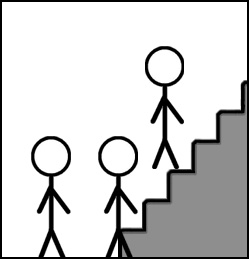
Figure 1.19 – Climbing stairs without locomotion
First, we play the walk animation and move the player forward. But now, the character is penetrating the surface. So, the collision detection system pulls the character above the surface to stop this impossible configuration.
Now, let's look at how we walk upstairs in reality. We put our foot firmly on the staircase and, using force, we pull the rest of our body onto the next step. However, it's not simple to implement this level of realism in games. We'll need many animations for different scenarios, including climbing ladders, walking/running upstairs, and so on. So, in the past, only the large studios with many animators could pull this off. Nowadays, however, we have automated systems for this:
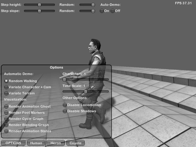
Figure 1.20 – Unity extension for inverse kinematics
This system can automatically blend our animated walk/run cycles and adjust the movements of the bones in the player's legs to ensure that the player's feet step on the ground correctly (in literature, this is called inverse kinematics). It can also adjust the animations that were initially designed for a specific speed and direction, to any speed and direction on any surface, such as steps and slopes. In Chapter 6, Path Following and Steering Behaviors, we'll learn how to use this locomotion system to apply realistic movement to our AI characters.


