Project 7 – Using the temperature sensor

The Nexys A7 board has an Analog Device ADT7420 temperature sensor. This chip uses an industry-standard I2C interface to communicate. This two-wire interface is used primarily for slower-speed devices. It has the advantage of allowing multiple chips to be connected through the same interface and be addressed individually. In our case, we will be using it to simply read the current temperature from the device and display the value on the seven-segment display.

Our first step will be to design an I2C interface. In Chapter 8, Introduction to AXI, we’ll be looking at designing a general-purpose I2C interface, but for now, we’ll use the fact that the ADT7420 comes up in a mode where we can get temperature data by reading two I2C memory locations. First, let’s look at the timing diagram for the I2C bus and the read cycle we’ll be using:

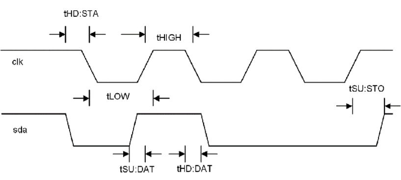
Figure 6.13: I2C timing

We can see from the timing diagram in Figure 6.13 that we have setup and hold times, which we have seen before relative to our own designs. We also have minimum clock widths we need to maintain. We can define parameters to handle these.

You can find the following code in the CH6/SystemVerilog/hdl/i2c_temp.sv folder:

localparam TIME_1SEC   = int'(INTERVAL/CLK_PER); // Clock ticks in 1 sec
localparam TIME_THDSTA = int'(600/CLK_PER);
localparam TIME_TSUSTA = int'(600/CLK_PER);
localparam TIME_THIGH  = int'(600/CLK_PER);
localparam TIME_TLOW   = int'(1300/CLK_PER);
localparam TIME_TSUDAT = int'(20/CLK_PER);
localparam TIME_TSUSTO = int'(600/CLK_PER);
localparam TIME_THDDAT = int'(30/CLK_PER);

Or, you can find the following code in the CH6/VHDL/hdl/i2c_temp.vhd folder:

constant TIME_1SEC   : integer          := INTERVAL / CLK_PER; -- Clock ticks in 1 sec
constant TIME_THDSTA : integer          := 600 / CLK_PER;
constant TIME_TSUSTA : integer          := 600 / CLK_PER;
constant TIME_THIGH  : integer          := 600 / CLK_PER;
constant TIME_TLOW   : integer          := 1300 / CLK_PER;
constant TIME_TSUSTO : integer          := 600 / CLK_PER;
constant TIME_THDDAT : integer          := 30 / CLK_PER;

1. I would encourage you to look at the state machine in the i2c_temp module in SystemVerilog or VHDL. The state machine controls the access to the temperature sensor on the Nexys A7 board. It’s fairly straightforward:
2. Wait for 1 second.
3. Send the start pattern on the Serial Data (SDA)/ Serial Clock (SCL) wires. This sends out the read command consisting of the 8-bit device address, the read bit plus the register address to the temperature sensor, and then reads back the 2 8-bit registers that contain the current temperature in Celsius.
4. Iterate until we have transmitted and received the data back.
5. Stop the transfer and go back to Step 1.

To access the temperature sensor, we’ve defined three buses:

1. Send the predefined start, device address, read bit, and stop signals.
2. Force the bus to tristate during the ACK cycles and data cycles.
3. Capture the data from the SDA bus.

The state machine provides us with access to the temperature sensor itself and returns the data. Now, we’ll need to find a way to display the data so a human can understand it.

Processing and displaying the data

We need to determine how best to display the temperature. The ADT7420 returns the data as a 16-bit fixed point value:

[15:7] Integer
[6:3] fraction * 0.0625
[2:0] Don't Care

Fixed point values are a user-defined type as there is no standard for representation. We’ll often refer to fixed point numbers as integer fractions. The ADT7420 outputs its temperature values as a 9.4 representation. We will discuss fixed-point math in more detail in the next section.

We can use our bin_to_bcd function on the integer portion to generate our seven-segment display data, but what can we do to calculate the fractional portion? We only have 16 values, so we could create a lookup table and simply look up the lower 4 digits. This is effectively creating ROM that can be indexed. ROM is created much like RAM:

SystemVerilog

logic [15:0] fraction_table[16];
initial begin
  for (int i = 0; i < 16; i++) fraction_table[i] = i*625;
end

VHDL

type slv16_array_t is array (0 to 15) of std_logic_vector(15 downto 0);
constant FRACTION_TABLE : slv16_array_t := (
  0  => std_logic_vector(to_unsigned(0 * 625, 16)),
  1  => std_logic_vector(to_unsigned(1 * 625, 16)),
  ...
  15 => std_logic_vector(to_unsigned(15 * 625, 16)));

In the preceding VHDL code, we have written out the sixteen array entries. While this may be acceptable for small, simple array constants, it is quite verbose and not very flexible. A better way to do this would be to initialize the constant with the return value of a function that computes the array elements:

VHDL

constant FRACTION_TABLE : slv16_array_t := init_fraction_table();

We can then convert the temperature based on the output of the temperature sensor chip:

SystemVerilog

// convert temperature from
  always @(posedge clk) begin
    digit_point  <= 8'b00010000;
    if (smooth_convert) begin
      if (smooth_data < 0) begin
        // negative values saturate at 0
        encoded_int  <= '0;
        fraction     <= '0;
      end else begin
        encoded_int  <= bin_to_bcd(smooth_data[15:7]); // Decimal portion
        fraction     <= bin_to_bcd(fraction_table[smooth_data[6:3]]);
      end
    end
  end // always @ (posedge clk)
  assign encoded = {encoded_int[3:0], fraction[3:0]};

VHDL

-- Convert temperature from binary to BCD
process(clk)
  variable sd_int : integer range 0 to 15;
begin
  if rising_edge(clk) then
    if smooth_convert then
      encoded_int  <= bin_to_bcd(23d"0" & smooth_data(15 downto 7)); -- integer portion
      sd_int       := to_integer(unsigned(smooth_data(6 downto 3)));
      encoded_frac <= bin_to_bcd(16d"0" & FRACTION_TABLE(sd_int)); -- fractional portion
      digit_point  <= "00010000";
    end if;
  end if;
end process;

One disadvantage of converting the temperature every second and having fractional precision is that the display will change quite a bit depending on your environment. We can apply what is essentially a filter to the data so that we take the average temperature over a period of time.

Now that we have learned how to handle the data, let’s learn more about how we can filter and improve the quality of that data by applying a smoothing function.

Smoothing out the data (oversampling)

In base 10, it’s very inexpensive to divide by a multiple of 10. Every multiple of 10 is simply a shift to the right of 1 digit:

12345 / 10  = 1234.5 Truncated = 1234, Rounded = 1235
12345 / 100 = 123.45 Truncated = 123,  Rounded = 123

Similarly, in binary, every shift to the right is a division by 2:

10110 >> 1 = 1011.0 Truncated = 1011, Rounded = 1011
10110 >> 2 = 101.10 Truncated = 101,  Rounded = 110

How does this help us with filtering? If we want to filter over a period of 2, 4, 8, 16, 32… 2ⁿ samples, the division operation is virtually free since it is simply a shift and possible rounding.

We can create a simple filter by summing our temperature data over a period of time:

Figure 6.14: Simple moving average filter

The way we create a moving average filter is to keep a running average over a period of time. In the preceding case, I picked 16 cycles, although any power of 2 is a good choice. A non-power of two is an option, but until we discuss how to improve this filter in Chapter 7, Math, Parallelism, and Pipelined Design, I wouldn’t consider it.

The way the filter works is that we add incoming data to an accumulator and subtract the input from 16 previous clock cycles. The accumulator then contains the sum of the incoming data over the last 16 cycles. If we divide this by 16 (right shift by 4 bits), we have an average over the last 16 cycles.

A deeper dive into FIFOs

The heart of a FIFO is RAM, a read and a write pointer, and flag generation logic. In a synchronous FIFO, it is very easy to implement:

Figure 6.15: Synchronous FIFO

The write pointer increments on every push and the read pointer increments on every pop.

Generating the flags boils down to comparing the read and write pointers against one another. When we are dealing with a synchronous FIFO, these comparisons are easy since everything is generated by the same clock and is properly timed. What about an asynchronous FIFO, that is, a FIFO with separate read and write clocks?

Remember our discussions on synchronization and multi-bit buses. What happens if we try to compare a read-and-write address on different clocks?

Figure 6.16: Asynchronous FIFO (non-functional)

The difference between a synchronous FIFO and an asynchronous FIFO is shown by the dotted line down the middle of Figure 6.16. Each half is an independent clock domain. In Figure 6.15, everything is on a single clock domain.

Let’s consider a read and write pointer on different clock domains. Assume the clocks have no relationship and that the depth of the FIFO is 16 with 4-bit addresses:

Figure 6.17: FIFO addressing

Looking at the preceding diagram, you can see that when the counter has multiple bits changing at the same time and the clocks are asynchronous, we really can’t determine what the captured address will be.

We can fix this issue by Gray coding the address pointers.

Using Gray coding for passing counter values

Binary counts increment by adding a 1 to the lowest bit. This results in a count such as the following:

00 – 01 – 10 – 11

Gray coding only allows one bit to change at a time, such as the following sequence:

00 – 01 – 11 – 10

Gray-coded counters have a limited range as they must always only have one-bit change at a time. A power of 2 is always safe to implement, but other combinations, such as 2ⁿ + 2^m, also work.

Let’s look at a FIFO using a Gray code:

Figure 6.18: Asynchronous FIFO with Gray coding

By adding a Gray code module and synchronizers across each clock domain, we can compare the gray-coded values against each other or convert them back to binary on the destination clock.

Since Gray code only allows one bit to change at a time, we are guaranteed to either capture the old value or the new one and not capture a transitional value that would cause a FIFO empty, full, or word count error.

Constraints

This is a case where we will want to utilize the set_max_delay constraint between the write pointer and the first register in the synchronizer:

Figure 6.19: Using set_max_delay

Looking at one side of the Gray code and synchronizer logic (there is a similar circuit on the read side), we can see where we need to apply the set max_delay timing constraint:

Set_max_delay -datapath_only <delay> -from [get_pins FF0/Q] -to [get_pins FF1/D] -datapath_only

To be absolutely safe, the delay should be set to the destination clock period or less. It can be up to 2 destination clocks, but to be safe, use between 1 and 1.5 times the destination clock period.

Generating our FIFO

We will be using a synchronous FIFO, but understanding how an asynchronous FIFO works is of critical importance if you decide to pursue a career utilizing FPGAs. You will almost certainly be asked an interview question regarding this.

We have the advantage that Xilinx has created a macro for us to use, xpm_fifo_(sync | async). You can view the instantiation in i2c_temp.sv. You’ll see that there are a lot of ports that we are not using (I’ve left them disconnected in the VHDL version). We’ll simply be pushing data into the FIFO on every convert signal and we have a small state machine that generates our data to be converted to send to our seven-segment display interface:

Figure 6.20: Simple temperature filter state machine

We can look at the state machine and see that it’s very straightforward. We create an elastic buffer using the FIFO to hold 16 samples. As each new sample comes in, we build up our accumulator value. When we hit 16 samples, we divide the accumulator by 16 and that gives us the average temperature over the previous 16 seconds:

SystemVerilog

localparam SMOOTHING_SHIFT = $clog2(SMOOTHING);
...
always @(posedge clk) begin
  rden           <= '0;
  rden_del       <= rden;
  smooth_convert <= '0;
  if (convert) begin
    smooth_count              <= smooth_count + 1'b1;
    accumulator               <= accumulator + unsigned'({temp_data[15:3], 3'b0});
  end else if (smooth_count == SMOOTHING+1) begin
    rden                    <= '1;
    smooth_count            <= smooth_count - 1'b1;
    accumulator             <= accumulator - signed'(dout);
  end else if (rden) begin
    smooth_data             <= accumulator >>> SMOOTHING_SHIFT;
    smooth_convert          <= '1;
  end
end

VHDL

smooth : process(clk)
  constant SMOOTHING_SHIFT : natural := natural(log2(real(SMOOTHING))); -- number of bits to shift to implement division by SMOOTHING factor
begin
  if rising_edge(clk) then
    rden           <= '0';
    smooth_convert <= '0';
    if convert then
      smooth_count <= smooth_count + 1;
      accumulator  <= accumulator + (unsigned(temp_data(temp_data'high downto 3)) & 3d"0");
    elsif smooth_count = SMOOTHING + 1 then
      rden         <= '1';
      smooth_count <= smooth_count - 1;
      accumulator  <= accumulator - unsigned(dout);
    elsif rden then
      smooth_convert <= '1';
      smooth_data    <= std_logic_vector(shift_right(accumulator, SMOOTHING_SHIFT)(smooth_data'range));
    end if;
  end if;
end process;

Take a look at the preceding code and see whether you can pick out the state progression. It’s not written as we have written it before, but you should be able to make out the flow. Once you’ve had a chance to look over the code, build it and try it out on the board.

One thing that may be a surprise is that the output stays 0 for a long period of time, 16 seconds to be precise. This is because we are waiting to fill the FIFO. What would happen if we output the accumulator/16 every cycle? Think about it for a minute or change the code and see.

If we always output accumulator/16, we would end up with a temperature creeping up from 1/16 of the current temperature to the average current temperature of the room. For something non-critical such as this, either method would be acceptable, but what if we didn’t want to do this and we always wanted the current value? For that, you’ll need to wait until Chapter 7, Math, Parallelism, and Pipelined Design, where we discuss fixed point representation.