Chapter 3: Feature Engineering
Activity 10: Calculating Time series Feature – Binning
Solution:
- Load the caret library:
#Time series features
library(caret)
#Install caret if not installed
#install.packages('caret')
- Load the GermanCredit dataset:
GermanCredit = read.csv("GermanCredit.csv")
duration<- GermanCredit$Duration #take the duration column
- Check the data summary as follows:
summary(duration)
The output is as follows:

Figure 3.27: The summary of the Duration values of German Credit dataset
- Load the ggplot2 library:
library(ggplot2)
- Plot using the command:
ggplot(data=GermanCredit, aes(x=GermanCredit$Duration)) +
geom_density(fill='lightblue') +
geom_rug() +
labs(x='mean Duration')
The output is as follows:

Figure 3.28: Plot of the duration vs density
- Create bins:
#Creating Bins
# set up boundaries for intervals/bins
breaks <- c(0,10,20,30,40,50,60,70,80)
- Create labels:
# specify interval/bin labels
labels <- c("<10", "10-20", "20-30", "30-40", "40-50", "50-60", "60-70", "70-80")
- Bucket the datapoints into the bins.
# bucketing data points into bins
bins <- cut(duration, breaks, include.lowest = T, right=FALSE, labels=labels)
- Find the number of elements in each bin:
# inspect bins
summary(bins)
The output is as follows:
summary(bins)
<10 10-20 20-30 30-40 40-50 50-60 60-70 70-80
143 403 241 131 66 2 13 1
- Plot the bins:
#Ploting the bins
plot(bins, main="Frequency of Duration", ylab="Duration Count", xlab="Duration Bins",col="bisque")
The output is as follows:
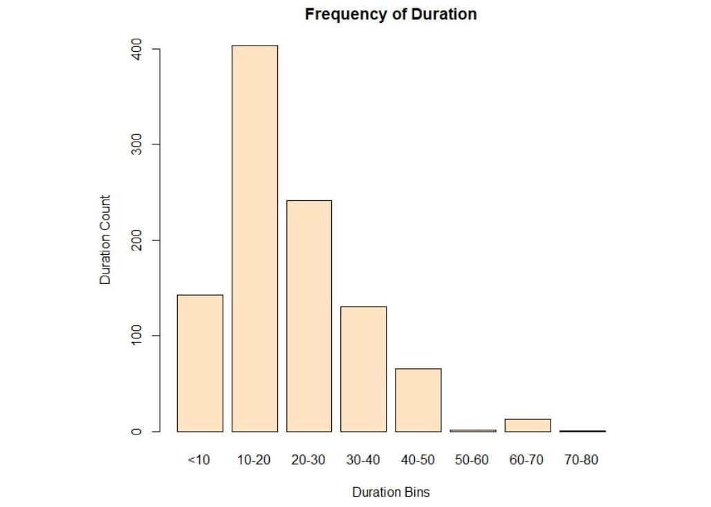
Figure 3.29: Plot of duration in bins
We can conclude that the maximum number of customers are within the range of 10 to 20.
Activity 11: Identifying Skewness
Solution:
- Load the library mlbench.
#Skewness
library(mlbench)
library(e1071)
- Load the PrimaIndainsDiabetes data.
PimaIndiansDiabetes = read.csv("PimaIndiansDiabetes.csv")
- Print the skewness of the glucose column, using the skewness() function.
#Printing the skewness of the columns
#Not skewed
skewness(PimaIndiansDiabetes$glucose)
The output is as follows:
[1] 0.1730754
- Plot the histogram using the histogram() function.
histogram(PimaIndiansDiabetes$glucose)
The output is as follows:

Figure 3.30: Histogram of the glucose values of the PrimaIndainsGlucose dataset
A negative skewness value means that the data is skewed to the left and a positive skewness value means that the data is skewed to the right. Since the value here is 0.17, the data is neither completely left or right skewed. Therefore, it is not skewed.
- Find the skewness of the age column using the skewness() function.
#Highly skewed
skewness(PimaIndiansDiabetes$age)
The output is as follows:
[1] 1.125188
- Plot the histogram using the histogram() function.
histogram(PimaIndiansDiabetes$age)
The output is as follows:
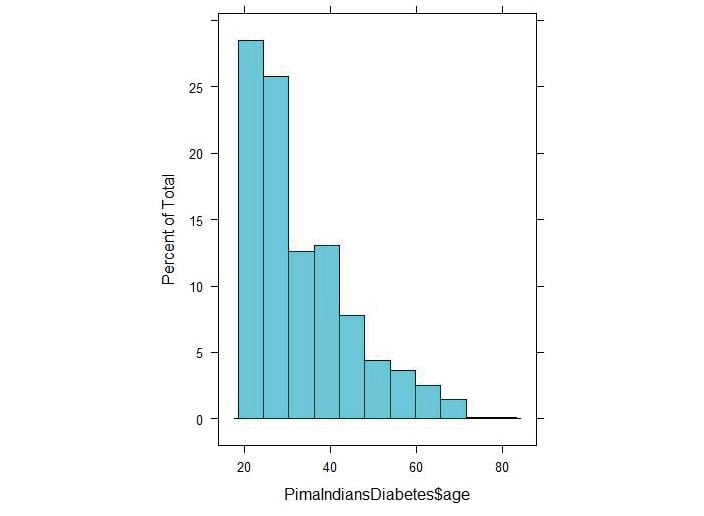
Figure 3.31: Histogram of the age values of the PrimaIndiansDiabetes dataset
The positive skewness value means that it is skewed to the right as we can see above.
Activity 12: Generating PCA
Solution:
- Load the GermanCredit data.
#PCA Analysis
data(GermanCredit)
- Create a subset of first 9 columns into another variable names GermanCredit_subset
#Use the German Credit Data
GermanCredit_subset <- GermanCredit[,1:9]
- Find the principal components:
#Find out the Principal components
principal_components <- prcomp(x = GermanCredit_subset, scale. = T)
- Print the principal components:
#Print the principal components
print(principal_components)
The output is as follows:
Standard deviations (1, .., p=9):
[1] 1.3505916 1.2008442 1.1084157 0.9721503 0.9459586
0.9317018 0.9106746 0.8345178 0.5211137
Rotation (n x k) = (9 x 9):

Figure 3.32: Histogram of the age values of the PrimaIndiansDiabetes dataset
Therefore, by using principal component analysis we can identify the top nine principal components in the dataset. These components are calculated from multiple fields and they can be used as features on their own.
Activity 13: Implementing the Random Forest Approach
Solution:
- Load the GermanCredit data:
data(GermanCredit)
- Create a subset to load the first ten columns into GermanCredit_subset.
GermanCredit_subset <- GermanCredit[,1:10]
- Attach the randomForest package:
library(randomForest)
- Train a random forest model using random_forest =randomForest(Class~., data=GermanCredit_subset):
random_forest = randomForest(Class~., data=GermanCredit_subset)
- Invoke importance() for the trained random_forest:
# Create an importance based on mean decreasing gini
importance(random_forest)
The output is as follows:
importance(random_forest)
MeanDecreaseGini
Duration 70.380265
Amount 121.458790
InstallmentRatePercentage 27.048517
ResidenceDuration 30.409254
Age 86.476017
NumberExistingCredits 18.746057
NumberPeopleMaintenance 12.026969
Telephone 15.581802
ForeignWorker 2.888387
- Use the varImp() function to view the list of important variables.
varImp(random_forest)
The output is as follows:
Overall
Duration 70.380265
Amount 121.458790
InstallmentRatePercentage 27.048517
ResidenceDuration 30.409254
Age 86.476017
NumberExistingCredits 18.746057
NumberPeopleMaintenance 12.026969
Telephone 15.581802
ForeignWorker 2.888387
In this activity, we built a random forest model and used it to see the importance of each variable in a dataset. The variables with higher scores are considered more important. Having done this, we can sort by importance and choose the top 5 or top 10 for the model or set a threshold for importance and choose all the variables that meet the threshold.
Activity 14: Selecting Features Using Variable Importance
Solution:
- Install the following packages:
install.packages("rpart")
library(rpart)
library(caret)
set.seed(10)
- Load the GermanCredit dataset:
data(GermanCredit)
- Create a subset to load the first ten columns into GermanCredit_subset:
GermanCredit_subset <- GermanCredit[,1:10]
- Train an rpart model using rPartMod <- train(Class ~ ., data=GermanCredit_subset, method="rpart"):
#Train a rpart model
rPartMod <- train(Class ~ ., data=GermanCredit_subset, method="rpart")
- Invoke the varImp() function, as in rpartImp <- varImp(rPartMod).
#Find variable importance
rpartImp <- varImp(rPartMod)
- Print rpartImp.
#Print variable importance
print(rpartImp)
The output is as follows:
rpart variable importance
Overall
Amount 100.000
Duration 89.670
Age 75.229
ForeignWorker 22.055
InstallmentRatePercentage 17.288
Telephone 7.813
ResidenceDuration 4.471
NumberExistingCredits 0.000
NumberPeopleMaintenance 0.000
- Plot rpartImp using plot().
#Plot top 5 variable importance
plot(rpartImp, top = 5, main='Variable Importance')
The output is as follows:
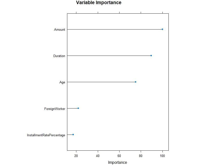
Figure 3.33: Variable importance for the fields
From the preceding plot, we can observe that Amount, Duration, and Age have high importance values.


