Time series forecasting with the functime library

Time series forecasting is a form of predictive analytics for time series data. It is to predict the future values based on historical data using statistical models. functime is a machine learning library for time series forecasting and feature extraction in Polars. It enables you to build time series forecasting models utilizing the Polars speed. functime is the Polars’ version of tsfresh, the popular time series feature extraction library.

In this recipe, we’ll cover how to build a simple time series forecasting model with the functime library, including feature extraction and plotting.

Important

As of the time of writing, Polars just upgraded to version 1.0.0 and functime has some compatibility issues with it. You may encounter an error after step 2; however, you can run those later steps with Polars version 0.20.31 (you’ll also need to change lf.collect_schema().names() to lf.columns for the code in step 1). If functime resolved the compatibility issues by the time you’re reading this, you can run all the steps in this recipe without issues.

Getting ready

Install the functime library with pip:

pip install functime

Note that functime has several dependencies including FLAML, scikit-learn, scipy, cloudpickle, holidays, and joblib.

In this recipe, we’ll use a different dataset based on the same data source, containing temperature data from multiple cities such as Toronto, New York, and Seattle. The structure of the dataset stays the same and the only difference is that this dataset will have temperatures per city and datetime columns. This kind of structure is called panel data, involving multiple time series data stacked on top of each other. It consists of multiple entity columns (city and datetime) and observed values (temperature). functime is designed to build forecasting models on panel data.

Reading the data in a LazyFrame is done as follows:

lf = pl.scan_csv('../data/historical_temperatures.csv', try_parse_dates=True)
lf.head().collect()

The preceding code will return the following output:

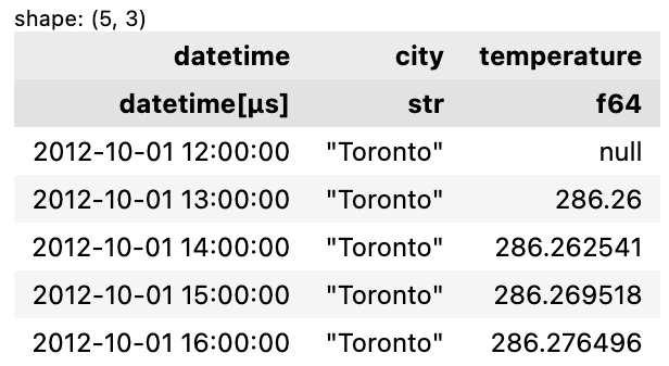
Figure 9.23 – The first five rows in the panel data

Let’s check the values in the city column:

lf.select('city').unique().sort('city').collect()

The preceding code will return the following output:

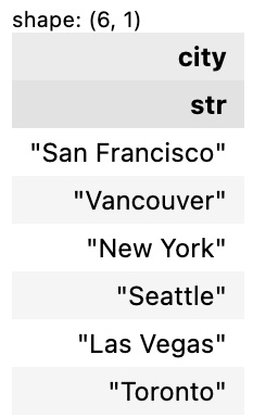
Figure 9.24 – Unique cities in the city column

You can also use .group_by() in combination with .head() or .tail() to check the first n rows for every value in the group-by column:

lf.group_by('city').head(3).collect()

The preceding code will return the following output:

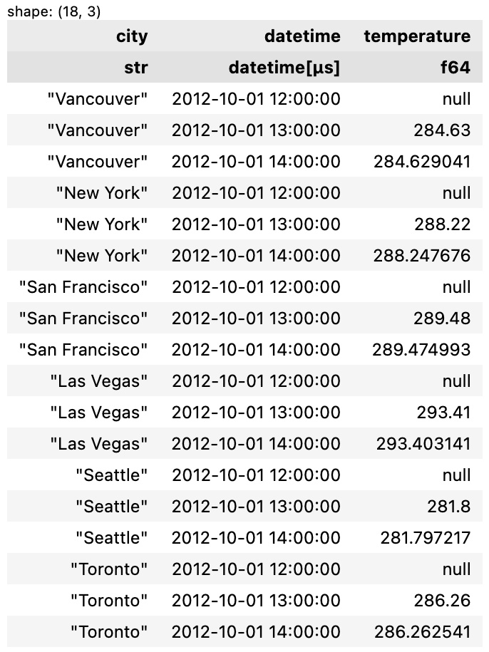
Figure 9.25 – The first n rows for every value in the group-by column (city)

How to do it...

Here’s how to build a forecasting model with functime.

1. Prepare the data at the month level as well as converting the temperature from Kelvin to Celsius:

   time_col, entity_col, value_col = lf.collect_schema().names()
   y = (
       lf
       .group_by_dynamic(
           time_col,
           every='1mo',
           group_by=entity_col,
       )
       .agg(
           (pl.col('temperature').mean()-273.15).round(1),
       )
   )
   y.group_by('city').head(3).collect()

The preceding code will return the following output:

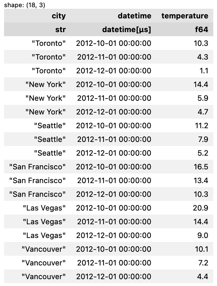
Figure 9.26 – The first n rows for every city with datetime and temperature converted

1. Split the dataset into training and testing sets. functime has similar syntax to scikit-learn for the train-test split:

   def create_train_test_sets(
       y,
       entity_col,
       time_col,
       test_size):
       from functime.cross_validation import train_test_split
       X = y.select(entity_col, time_col)
       y_train, y_test = (
           y
           .select(entity_col, time_col, value_col)
           .pipe(train_test_split(test_size))
       )
       X_train, X_test = X.pipe(train_test_split(test_size))
       return X_train, X_test, y_train, y_test
   test_size = 3
   X_train, X_test, y_train, y_test = create_train_test_sets(y, entity_col, time_col, test_size)

2. Predict the values and calculate the Mean Absolute Scaled Error (MASE) metric for the model:

   def predict_with_linear_model(
       lags,
       freq,
       y_train,
       fh
   ):
       from functime.forecasting import linear_model
       forecaster = linear_model(lags=lags, freq=freq)
       forecaster.fit(y=y_train)
       y_pred = forecaster.predict(fh=fh)
       return y_pred
   y_pred = predict_with_linear_model(24, '1mo', y_train, test_size)
   from functime.metrics import mase
   scores = mase(y_true=y_test, y_pred=y_pred, y_train=y_train)
   display(y_pred, scores)

   The preceding code will return the following output:

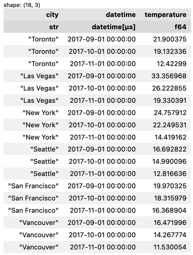
Figure 9.27 – Forecasted/predicated values

And here’s the MASE values:

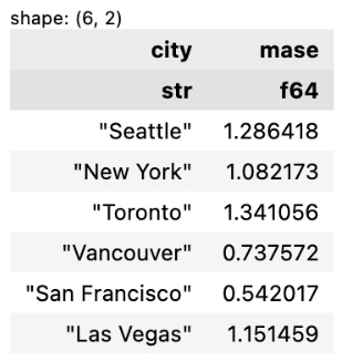
Figure 9.28 – MASE values for each city

3. Visualizing the predicted values and the original data using hvplot is done as follows:

   actual_viz = (
       y
       .collect()
       .plot.line(
           x='datetime', y='temperature', by='city', subplots=True
       )
       .cols(2)
   )
   pred_viz = (
       y_pred
       .plot.line(
           x='datetime', y='temperature', by='city', subplots=True
       )
       .cols(2)
   )
   actual_viz * pred_viz

   The preceding code will return the following output:

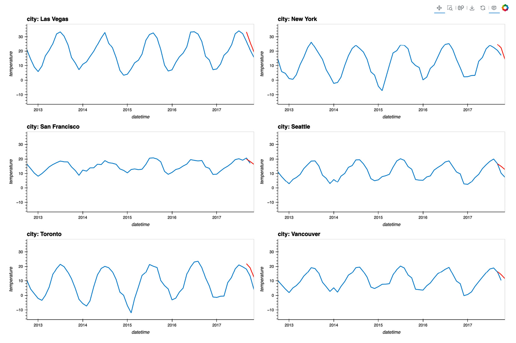
Figure 9.29 - Original values and predicated values visualized in line charts

How it works...

As you saw, building a forecasting model with functime is not complicated at all, especially if you have some experience with other forecasting libraries. The process of creating training and testing sets looks very much like how you do it in scikit-learn.

You might’ve noticed the use of the .pipe() method in step 2. It can take user-defined functions (UDFs) in sequence so that your code is more structured.

For feature extraction, functime provides the custom ts namespace that contains every feature. The ts namespace can be used just like other namespaces such as str and list. They allow you to access useful methods in any Polars expression. We’ll see an example of extracting features using the ts namespace shortly.

There is more...

Here’s an example of how to extract features in functime:

from functime.seasonality import add_calendar_effects
y_features = (
    lf
    .group_by_dynamic(
        time_col,
        every='1mo',
        by=entity_col,
    )
    .agg(
        (pl.col('temperature').mean()-273.15).round(1),
        pl.col(value_col).ts.binned_entropy(bin_count=10)
        .alias('binned_entropy'),
        pl.col(value_col).ts.lempel_ziv_complexity(threshold=3)
        .alias('lempel_ziv_complexity'),
        pl.col(value_col).ts.longest_streak_above_mean()
        .alias('longest_streak_above_mean')
    )
    .pipe(add_calendar_effects(['month']))
)
y_features.head().collect()

The preceding code will return the following output:

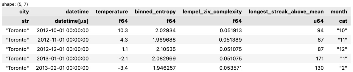
Figure 9.30 – Data with extracted features

In the preceding code, note that the add_calendar_effects() function adds a month column. The seasonality API provides functions to extract calendar/holiday effects and Fourier features for time series seasonality.

See also

Please refer to the functime documentation to learn more:

• https://docs.functime.ai/user-guide/forecasting/
• https://docs.functime.ai/user-guide/feature-extraction/
• https://docs.functime.ai/user-guide/seasonality/