Search icon CANCEL
Subscription
0
Cart icon
Your Cart (0 item)
Close icon
You have no products in your basket yet
Save more on your purchases now! discount-offer-chevron-icon
Savings automatically calculated. No voucher code required.
Arrow left icon
Explore Products
Best Sellers
New Releases
Books
Videos
Audiobooks
Learning Hub
Conferences
Free Learning
Arrow right icon
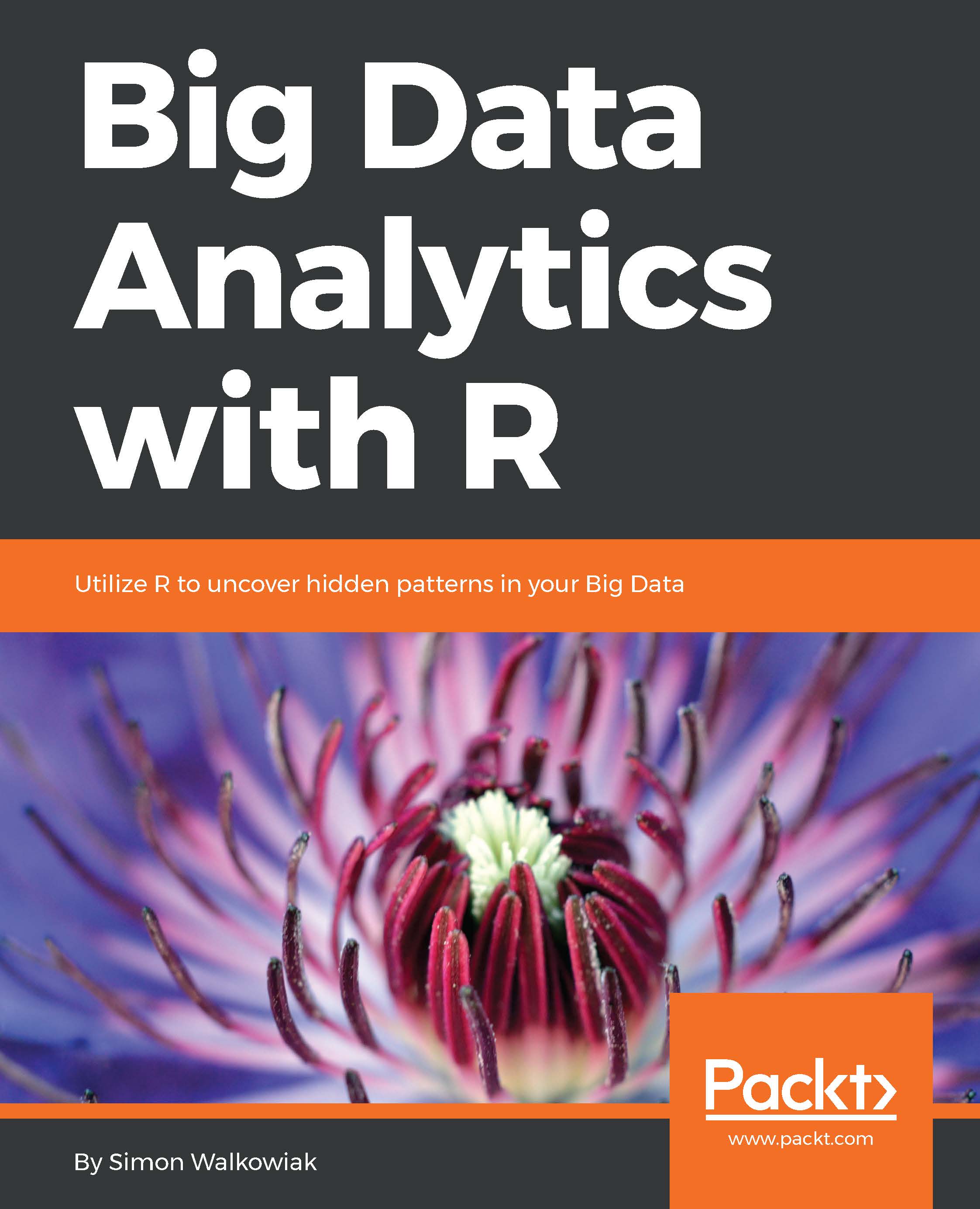
Big Data Analytics with R

Big Data Analytics with R: Leverage R Programming to uncover hidden patterns in your Big Data

eBook
$32.99 $47.99
Paperback
$60.99
Subscription
Free Trial
Renews at $19.99p/m

What do you get with Print?

Product feature icon Instant access to your digital eBook copy whilst your Print order is Shipped
Product feature icon Paperback book shipped to your preferred address
Product feature icon Download this book in EPUB and PDF formats
Product feature icon Access this title in our online reader with advanced features
Product feature icon DRM FREE - Read whenever, wherever and however you want
OR
Modal Close icon
Payment Processing...
tick Completed

Shipping Address

Billing Address

Shipping Methods
Table of content icon View table of contents Preview book icon Preview Book

Big Data Analytics with R

Big Data – The monster re-defined

Every time Leo Messi scores at Camp Nou in Barcelona, almost one hundred thousand Barca fans cheer in support of their most prolific striker. Social media services such as Twitter, Instagram, and Facebook are instantaneously flooded with comments, views, opinions, analyses, photographs, and videos of yet another wonder goal from the Argentinian goalscorer. One such goal, scored in the semifinal of the UEFA Champions League, against Bayern Munich in May 2015, generated more than 25,000 tweets per minute in the United Kingdom alone, making it the most tweeted sports moment of 2015 in this country. A goal like this creates a widespread excitement, not only among football fans and sports journalists. It is also a powerful driver for the marketing departments of numerous sportswear stores around the globe, who try to predict, with a military precision, day-to-day, in-store, and online sales of Messi's shirts, and other FC Barcelona related memorabilia. At the same time, major TV stations attempt to outbid each other in order to show forthcoming Barca games, and attract multi-million revenues from advertisement slots during the half-time breaks. For a number of industries, this one goal is potentially worth much more than Messi's 20 million Euro annual salary. This one moment also creates an abundance of information, which needs to be somehow collected, stored, transformed, analyzed, and redelivered in the form of yet another product, for example, sports news with a slow-motion replay of Messi's killing strike, additional shirts dispatched to sportswear stores, or a sales spreadsheet and a marketing briefing outlining Barca's TV revenue figures.

Such moments, like memorable Messi's goals against Bayern Munich, happen on a daily basis. Actually, they are probably happening right now, while you are holding this book in front of your eyes. If you want to check what currently makes the world buzz, go to the Twitter web page and click on the Moments tab to see the most trending hashtags and topics at this very moment. Each of these less, or more, important events generates vast amounts of data in many different formats, from social media status updates to YouTube videos and blog posts to mention just a few. These data may also be easily linked with other sources of the event-related information to create complex unstructured deposits of data that attempt to explain one specific topic from various perspectives and using different research methods. But here is the first problem: the simplicity of data mining in the era of the World Wide Web means that we can very quickly fill up all the available storage on our hard drives, or run out of processing power and memory resources to crunch the collected data. If you end up having such issues when managing your data, you are probably dealing with something that has been vaguely denoted as Big Data.

Big Data is possibly the scariest, deadliest and the most frustrating phrase which can ever be heard by a traditionally trained statistician or a researcher. The initial problem lies in how the concept of Big Data is defined. If you ask ten, randomly selected, students what they understand by the term Big Data they will probably give you ten, very different, answers. By default, most will immediately conclude that Big Data has something to do with the size of a data set, the number of rows and columns; depending on their fields they will use similar wording. Indeed they will be somewhat correct, but it's when we inquire about when exactly normal data becomes Big that the argument kicks off. Some (maybe psychologists?) will try to convince you that even 100 MB is quite a big file or big enough to be scary. Some others (social scientists?) will probably say that 1 GB heavy data would definitely make them anxious. Trainee actuaries, on the other hand, will suggest that 5 GB would be problematic, as even Excel suddenly slows down or doesn't want to open the file. In fact, in many areas of medical science (such as human genome studies) file sizes easily exceed 100 GB each, and most industry data centers deal with data in the region of 2 TB to 10 TB at a time. Leading organizations and multi-billion dollar companies such as Google, Facebook, or YouTube manage petabytes of information on a daily basis. What is then the threshold to qualify data as Big?

The answer is not very straightforward, and the exact number is not set in stone. To give an approximate estimate we first need to differentiate between simply storing the data, and processing or analyzing the data. If your goal was to preserve 1,000 YouTube videos on a hard drive, it most likely wouldn't be a very demanding task. Data storage is relatively inexpensive nowadays, and new rapidly emerging technologies bring its prices down almost as you read this book. It is amazing just to think that only 20 years ago, $300 would merely buy you a 2GB hard drive for your personal computer, but 10 years later the same amount would suffice to purchase a hard drive with a 200 times greater capacity. As of December 2015, having a budget of $300 can easily afford you a 1TB SATA III internal solid-state drive: a fast and reliable hard drive, one of the best of its type currently available to personal users. Obviously, you can go for cheaper and more traditional hard disks in order to store your 1,000 YouTube videos; there is a large selection of available products to suit every budget. It would be a slightly different story, however, if you were tasked to process all those 1,000 videos, for example by creating shorter versions of each or adding subtitles. Even worse if you had to analyze the actual footage of each movie, and quantify, for example, how many seconds per video red colored objects of the size of at least 20x20 pixels are shown. Such tasks do not only require considerable storage capacities, but also, and primarily, the processing power of the computing facilities at your disposal. You could possibly still process and analyze each video, one by one, using a top-of-the-range personal computer, but 1,000 video files would definitely exceed its capabilities and most likely your limits of patience too. In order to speed up the processing of such tasks, you would need to quickly find some extra cash to invest into further hardware upgrades, but then again this would not solve the issue. Currently, personal computers are only vertically scalable to a very limited extent. As long as your task does not involve heavy data processing, and is simply restricted to file storage, an individual machine may suffice. However, at this point, apart from large enough hard drives, we would need to make sure we have a sufficient amount of Random Access Memory (RAM), and fast, heavy-duty processors on compatible motherboards installed in our units. Upgrades of individual components, in a single machine, may be costly, short-lived due to rapidly advancing new technologies, and unlikely to bring a real change to complex data crunching tasks. Strictly speaking, this is not the most efficient and flexible approach for Big Data analytics to say the least. A couple of sentence back, I used the plural units intentionally, as we would most probably have to process the data on a cluster of machines working in parallel. Without going into details at this stage, the task would require our system to be horizontally scalable, meaning that we would be capable of easily increasing (or decreasing) the number of units (nodes) connected in our cluster as we wish. A clear advantage of horizontal scalability over vertical scalability is that we would simply be able to use as many nodes working in parallel as required by our task, and we would not be bothered too much with the individual configuration of each and every machine in our cluster.

Let's go back now for a moment to our students and the question of when normal data becomes Big? Amongst the many definitions of Big Data, one is particularly neat and generally applicable to a very wide range of scenarios. One byte more than you are comfortable with is a well-known phrase used by Big Data conference speakers, but I can't deny that it encapsulates the meaning of Big Data very precisely, and yet it is non-specific enough it leaves the freedom to make a subjective decision to each one of us as to what and when to qualify data as Big. In fact, all our students, whether they said Big Data was as little as 100MB or as much as 10 petabytes, were more or less correct in their responses. As long as an individual (and his/her equipment) is not comfortable with a certain size of data, we should assume that this is Big Data for them. The size of data is not, however, the only factor that makes the data Big. Although the simplified definition of Big Data, previously presented, explicitly refers to the one byte as a measurement of size, we should dissect the second part of the statement, in a few sentences, to have a greater understanding of what Big Data actually means. Data do not just come to us and sit in a file. Nowadays, most data change, sometimes very rapidly. Near real-time analytics of Big Data currently gives huge headaches to in-house data science departments, even at international large financial institutions or energy companies. In fact stock-market data, or sensor data, are pretty good, but still quite extreme examples of high-dimensional data that are stored and analyzed at milliseconds intervals. Several seconds of delay in producing data analyses, on near real-time information, may cost investors quite substantial amounts, and result in losses in their portfolio value, so the speed of processing fast-moving data is definitely a considerable issue at the moment. Moreover, data are now more complex than ever before. Information may be scrapped off the websites as unstructured text, JSON format, HTML files, through service APIs, and so on. Excel spreadsheets and traditional file formats such as Comma-Separated Values (CSV) or tab-delimited files that represent structured data are not in the majority any more. It is also very limiting to think of data as of only numeric or textual types. There is an enormous variety of available formats that store, for instance, audio and visual information, graphics, sensors, and signals, 3D rendering and imaging files, or data collected and compiled using highly specialized scientific programs or analytical software packages such as Stata or Statistical Package for the Social Sciences (SPSS) to name just a few (a large list of most available formats is accessible through Wikipedia at https://en.wikipedia.org/wiki/List_of_file_formats ).

The size of data, the speed of their inputs/outputs and the differing formats and types of data were in fact the original three Vs:  Volume, Velocity, and Variety, described in the article titled 3D Data Management: Controlling Data Volume, Velocity, and Variety published by Doug Laney back in 2001, as major conditions to treat any data as Big Data. Doug's famous three Vs were further extended by other data scientists to include more specific and sometimes more qualitative factors such as data variability (for data with periodic peaks of data flow), complexity (for multiple sources of related data), veracity (coined by IBM and denoting trustworthiness of data consistency), or value (for examples of insight and interpretation). No matter how many Vs or Cs we use to describe Big Data, it generally revolves around the limitations of the available IT infrastructure, the skills of the people dealing with large data sets and the methods applied to collect, store, and process these data. As we have previously concluded that Big Data may be defined differently by different entities (for example individual users, academic departments, governments, large financial companies, or technology leaders), we can now rephrase the previously referenced definition in the following general statement:

Big Data any data that cause significant processing, management, analytical, and interpretational problems.

Also, for the purpose of this book, we will assume that such problematic data will generally start from around 4 GB to 8 GB in size, the standard capacity of RAM installed in most commercial personal computers available to individual users in the years 2014 and 2015. This arbitrary threshold will make more sense when we explain traditional limitations of the R language later on in this chapter, and methods of Big Data in-memory processing across several chapters in this book.

Big Data toolbox - dealing with the giant

Just like doctors cannot treat all medical symptoms with generic paracetamol and ibuprofen, data scientists need to use more potent methods to store and manage vast amounts of data. Knowing already how Big Data can be defined, and what requirements have to be met in order to qualify data as Big, we can now take a step forward and introduce a number of tools that are specialized in dealing with these enormous data sets. Although traditional techniques may still be valid in certain circumstances, Big Data comes with its own ecosystem of scalable frameworks and applications that  facilitate the processing and management of unusually large or fast data. In this chapter, we will briefly present several most common Big Data tools, which will be further explored in greater detail later on in the book.

Hadoop - the elephant in the room

If you have been in the Big Data industry for as little as one day, you surely must have heard the unfamiliar sounding word Hadoop, at least every third sentence during frequent tea break discussions with your work colleagues or fellow students. Named after Doug Cutting's child's favorite toy, a yellow stuffed elephant, Hadoop has been with us for nearly 11 years. Its origins began around the year 2002 when Doug Cutting was commissioned to lead the Apache Nutch project-a scalable open source search engine. Several months into the project, Cutting and his colleague Mike Cafarella (then a graduate student at University of Washington) ran into serious problems with the scaling up and robustness of their Nutch framework owing to growing storage and processing needs. The solution came from none other than Google, and more precisely from a paper titled The Google File System authored by Ghemawat, Gobioff, and Leung, and published in the proceedings of the 19th ACM Symposium on Operating Systems Principles. The article revisited the original idea of Big Files invented by Larry Page and Sergey Brin, and proposed a revolutionary new method of storing large files partitioned into fixed-size 64 MB chunks across many nodes of the cluster built from cheap commodity hardware. In order to prevent failures and improve efficiency of this setup, the file system creates copies of chunks of data, and distributs them across a number of nodes, which were in turn mapped and managed by a master server. Several months later, Google surprised Cutting and Cafarella with another groundbreaking research article known as MapReduce: Simplified Data Processing on Large Clusters, written by Dean and Ghemawat, and published in the Proceedings of the 6th Conference on Symposium on Operating Systems Design and Implementation.

The MapReduce framework became a kind of mortar between bricks, in the form of data distributed across numerous nodes in the file system, and the outputs of data transformations and processing tasks.

The MapReduce model contains three essential stages. The first phase is the Mapping procedure, which includes indexing and sorting data into the desired structure based on the specified key-value pairs of the mapper (that is, a script doing the mapping). The Shuffle stage is responsible for the redistribution of the mapper's outputs across nodes, depending on the key; that is, the outputs for one specific key are stored on the same node. The Reduce stage results in producing a kind of summary output of the previously mapped and shuffled data, for example, a descriptive statistic such as the arithmetic mean for a continuous measurement by each key (for example a categorical variable). A simplified data processing workflow, using the MapReduce framework in Google and Distributed File System, is presented in the following figure:

Hadoop - the elephant in the room
A diagram depicting a simplified Distributed File System architecture and stages of the MapReduce framework

The ideas of the Google File System model, and the MapReduce paradigm, resonated very well with Cutting and Cafarella's plans, and they introduced both frameworks into their own research on Nutch. For the first time their web crawler algorithm could be run in parallel on several commodity machines with minimal supervision from a human engineer.

In 2006, Cutting moved to Yahoo! and in 2008, Hadoop became a separate Nutch independent Apache project. Since then, it's been on a never-ending journey towards greater reliability and scalability to allow bigger and faster workloads of data to be effectively crunched by gradually increasing node numbers. In the meantime, Hadoop has also become available as an add-on service on leading cloud computing platforms such as Microsoft Azure, Amazon Elastic Cloud Computing (EC2), or Google Cloud Platform. This new, unrestricted, and flexible way of accessing shared and affordable commodity hardware, enabled numerous companies as well as individual data scientists and developers to dramatically cut their production costs and process larger than ever data in a more efficient and robust manner. A few Hadoop record-breaking milestones are worth mentioning at this point. In the well-known real-world example at the end of 2007, the New York Times was able to convert more than 4TB of images, within less than 24 hours, using a cluster built of 100 nodes on Amazon EC2, for as little as $200. A job that would have potentially taken weeks of hard labor, and a considerable amount of working man-hours, could now be achieved at a fraction of the original cost, in a significantly shorter scope of time. A year later 1TB of data was already sorted in 209 seconds and in 2009, Yahoo! set a new record by sorting the same amount of data in just 62 seconds. In 2013, Hadoop reached its best Gray Sort Benchmark ( http://sortbenchmark.org/ ) score so far. Using 2,100 nodes, Thomas Graves from Yahoo! was able to sort 102.5TB in 4,328 seconds, so roughly 1.42TB per minute.

In recent years, the Hadoop and MapReduce frameworks have been extensively used by the largest technology businesses such as Facebook, Google, Yahoo!, major financial and insurance companies, research institutes, and Academia, as well as Big Data individual enthusiasts. A number of enterprises offering commercial distributions of Hadoop such as Cloudera (headed by Tom Reilly with Doug Cutting as Chief Architect) or Hortonworks (currently led by Rob Bearden-a former senior officer at Oracle and CEO of numerous successful open source projects such as SpringSource and JBoss, and previously run by Eric Baldeschwieler-a former Yahoo! engineer working with Cutting) have spun off from the original Hadoop project, and evolved into separate entities, providing additional Big Data proprietary tools, and extending the applications and usability of Hadoop ecosystem. Although MapReduce and Hadoop revolutionized the way we process vast quantities of data, and hugely propagated Big Data analytics throughout the business world and individual users alike, they also received some criticism for their still present performance limitations, reliability issues, and certain programming difficulties. We will explore these limitations and explain other Hadoop and MapReduce features in much greater detail using practical examples in Chapter 4, Hadoop and MapReduce Framework for R.

Databases

There are many excellent online and offline resources and publications available to readers, on both SQL-based Relational Database Management System (RDBMS), and more modern non-relational and Not Only SQL (NoSQL) databases. This book will not attempt to describe each and every one of them with a high level of detail, but in turn it will provide you with several practical examples on how to store large amounts of information in such systems, carry out essential data crunching and processing of the data using known and tested R packages, and extract the outputs of these Big Data transformations from databases directly into your R session.

As mentioned earlier, in Chapter 5, R with Relational Database Management System (RDBMSs), we will begin with a very gentle introduction to standard and more traditional databases built on the relational model developed in 1970s by Oxford-educated English computer scientist Edgar Codd, while working at IBM's laboratories in San Jose. Don't worry if you have not got too much experience with databases yet. At this stage, it is only important for you to know that, in the RDBMS, the data is stored in a structured way in the form of tables with fields and records. Depending on the specific industry that you come from, fields can be understood as either variables or columns, and records may alternatively be referred to as observations or rows of data. In other words, fields are the smallest units of information and records are collections of these fields. Fields, like variables, come with certain attributes assigned to them, for example, they may contain only numeric or string values, double or long, and so on. These attributes can be set when inputting the data into the database. The RDBMS have proved extremely popular and most (if not all) currently functioning enterprises that collect and store large quantities of data have some sort of relational databases in place. The RDBMS can be easily queried using the Structured Query Language (SQL)-an accessible and quite natural database management programming language, firstly created at IBM by Donald Chamberlin and Raymond Boyce, and later commercialized and further developed by Oracle. Since the original birth of the first RDBMS, they have evolved into fully supported commercial products with Oracle, IBM, and Microsoft being in control of almost 90% of the total RDBMS market share. In our examples of R's connectivity with RDBMS ( Chapter 5, R with Relational Database Management System (RDBMSs)) we will employ a number of the most popular relational and open source databases available to users, including MySQL, PostgreSQL, SQLite, and MariaDB.

However, this is not where we are going to end our journey through the exciting landscape of databases and their Big Data applications. Although RDBMS perform very well in the cases of heavy transactional load, and their ability to process quite complex SQL queries is one of their greatest advantages, they are not so good with (near) real-time and streaming data. Also they generally do not support unstructured and hierarchical data, and they are not easily horizontally scalable. In response to these needs, a new type of database has recently evolved, or to be more precise, it was revived from a long state of inactivity as non-relational databases were known and in use, parallel with RDBMS, even forty years ago, but they never became as popular. NoSQL and non-relational databases, unlike SQL-based RDBMS, come with no predefined schema, thus allowing the users a much needed flexibility without altering the data. They generally scale horizontally very well and are praised for the speed of processing, making them ideal storage solutions for (near) real-time analytics in such industries as retail, marketing, and financial services. They also come with their own flavors of SQL like queries; some of them, for example, the MongoDB NoSQL language, are very expressive and allow users to carry out most data transformations and manipulations as well as complex data aggregation pipelines or even database-specific MapReduce implementations. The rapid growth of interactive web-based services, social media, and streaming data products resulted in a large array of such purpose-specific NoSQL databases being developed. In Chapter 6, R with Non-Relational and (NoSQL) Databases, we will present several examples of Big Data analytics with R using data stored in three leading open source non-relational databases: a popular document-based NoSQL, MongoDB, and a distributed Apache Hadoop-complaint HBase database.

Hadoop Spark-ed up

In the section Hadoop - the elephant in the room, we introduced you to the essential basics of Hadoop, its Hadoop Distributed File System (HDFS) and the MapReduce paradigm. Despite the huge popularity of Hadoop in both academic and industrial settings, many users complain that Hadoop is generally quite slow and some computationally demanding data processing operations can take hours to complete. Spark, which makes use of, and is deployed on top of, the existing HDFS, has been designed to excel in iterative calculations in order to fine-tune Hadoop's in-memory performance by up to 100 times faster, and about 10 times faster when run on disk.

Spark comes with its own small but growing ecosystem of additional tools and applications that support large-scale processing of structured data by implementing SQL queries into Spark programs (through Spark SQL), enabling fault-tolerant operations on streaming data (Spark Streaming), allowing users to perform sophisticated machine-learning models (MLlib), and carrying out out-of-the-box parallel community detection algorithms such as PageRank, label propagation, and many others on graphs and collections through the GraphX module. Owing to the open source, community-run Apache status of the project, Spark has already attracted an enormous interest from people involved in Big Data analysis and machine learning. As of the end of July 2016, there are over 240 third-party packages developed by independent Spark users available at the http://spark-packages.org/ website. A large majority of them allow further integration of Spark with other more or less common Big Data tools on the market. Please feel free to visit the page and check which tools or programming languages, that are known to you, are already supported by the packages indexed in the directory.

In Chapter 7, Faster than Hadoop: Spark and R and Chapter 8, Machine Learning for Big Data in R we will discuss the methods of utilizing Apache Spark in our Big Data analytics workflows using the R programming language. However before we do so, we need to familiarize ourselves with the most integral part of this book-the R language itself.

R – The unsung Big Data hero

By now you have been introduced to the notion of Big Data, its features, and its characteristics, as well as the most widely used Big Data analytics tools and frameworks such as Hadoop, HDFS, MapReduce framework, relational and non-relational databases, and Apache Spark project. They will be explored more thoroughly in the next few chapters of this book, but now the time has finally come to present the true hero and the main subject of this book-the R language. Although R as a separate language on its own has been with us since the mid 90s, it is derived from a more archaic S language developed by John Chambers in the mid 1970s. During Chambers' days in Bell Laboratories, one of the goals of his team was to design a user-friendly, interactive, and quick-in-deployment interface for statistical analysis and data visualizations. As they frequently had to deal with non-standard data analyses, and different data formats, the flexibility of this new tool, and its ability to make the most of the previously used Fortran algorithms, were the highest-order priorities. Also, the project was developed to implement certain graphical capabilities in order to visualize the outputs of numeric computations. The first version was run on a Honeywell operated machine, which wasn't the ideal platform, owing to a number of limitations and impracticalities.

The continuous work on S language progressed quite quickly and by 1981 Chambers and his colleagues were able to release a Unix implementation of the S environment along with a first book-cum-manual titled S: A Language and System for Data Analysis. In fact S was a hybrid-an environment or an interface allowing access to Fortran-based statistical algorithms through a set of built-in functions, operating on data with the flexibility of custom programmable syntax, for those users who wished to go beyond default statistical methods and implement more sophisticated computations. This hybrid, quasi object-oriented and functional programming language-like, statistical computing tool created a certain amount of ambiguity and confusion, even amongst its original developers. It is a well-known story that John Chambers, Richard Becker, and other Bell Labs engineers working on S at that time had considerable problems in categorizing their software as either a programming language, a system, or an environment. More importantly, however, S found a fertile ground in Academia and statistical research, which resulted in a sharp increase in external contributions from a growing community of S users. Future versions of S would enhance the functional and object-based structure of the S environment by allowing users to store their data, subsets, outputs of the computations, and even functions and graphs as separate objects. Also, since the third release of S in 1986, the core of the environment has been written in the C language, and the interface with Fortran modules has become accessible dynamically through the evaluator directly from S functions, rather than through a preprocessor and compilation, which was the case in the earlier versions. Of course, the new releases of the modernized and polished S environment were followed by a number of books authored by Chambers, Becker, and now also Allan Wilks, in which they explained the structure of the S syntax and frequently used statistical functions. The S environment laid the foundations for the R programming language, which has been further redesigned in 1990s by Robert Gentleman and Ross Ihaka from the University of Auckland in New Zealand. Despite some differences (a comprehensive list of differences between the S and R languages is available at https://cran.r-project.org/doc/FAQ/R-FAQ.html#R-and-S ), the code written in the S language runs almost unaltered in the R environment. In fact R and also the S-Plus language are the implementations of S-in its more evolved versions, and it is advisable to treat them as such. Probably the most striking difference between S and R, comes from the fact that R blended in an evaluation model based on the lexical scoping adopted from Steele and Sussman's Scheme programming language. The implementation of lexical scoping in R allowed you to assign free variables, depending on the environment in which a function referencing such variables was created, whereas in S free variables could have only been defined globally. The evaluation model used in R meant that the functions, in comparison with S, were more expressive and written in a more natural way giving the developers or analysts more flexibility and greater capabilities by defining variables specific to particular functions within their own environments. The link provided earlier, lists other minor, or very subtle, differences between both languages-many of which are sometimes not very apparent unless they are explicitly referred to in error messages when attempting to run a line of R code.

Currently, R comes in various shapes or forms, as there are several open source and commercial implementations of the language. The most popular, and the ones used throughout this book, are the free R GUI available to download from the R Project CRAN website at https://cran.r-project.org/ and our preferred and also free-of-charge RStudio IDE available from https://www.rstudio.com/ . Owing to their popularity and functionalities, both implementations deserve a few words of introduction.

The most generic R implementation is a free, open source project managed and distributed by the R Foundation for Statistical Computing headquartered in Vienna (Austria) at the Institute for Statistics and Mathematics. It is a not-for-profit organization, founded and set up by the members of the R Development Core Team, which includes a number of well-known academics in statistical research, R experts, and some of the most prolific R contributors over the past several years. Amongst its members, there are still the original fathers of the S and R languages such as John Chambers, Robert Gentleman, and Ross Ihaka, as well as the most influential R developers: Dirk Eddelbuettel, Peter Dalgaard, Bettina Grun, and Hadley Wickham to mention just a few. The team is responsible for the supervision and the management of the R core source code, approval of changes and alterations to the source code, and the implementation of community contributions. Through the web pages of the Comprehensive R Archive Network (CRAN) ( https://cran.r-project.org/ ), the R Development Core Team releases new versions of the R base installation and publishes recent third-party packages created by independent R developers and R community members. They also release research-oriented, open access, refereed periodic R Journals, and organize extremely popular annual useR! conferences, which regularly gather hundreds of passionate R users from around the world.

The R core is the basis for enterprise-ready open source and commercial license products developed by RStudio operating from Boston, MA and led by the Chief Scientist Dr. Hadley Wickham-a creator of numerous crucial data analysis and visualization packages for R, for example, ggplot2, rggobi, plyr, reshape, and many more. Their IDE is probably the best and most user-friendly R interface currently available to R users, and if you still don't have it, we recommend that you install it on your personal computer as soon as possible. The RStudio IDE consists of an easy-to-navigate workspace view, with a console window, and an editor, equipped with code highlighting and a direct code execution facility, as well as additional views allowing user-friendly control over plots and visualizations, file management within and outside the working directory, core and third-party packages, history of functions and expressions, management of R objects, code debugging functionalities, and also a direct access to help and support files.

As the R core is a multi-platform tool, RStudio is also available to users of the Windows, Mac, or Linux operating systems. We will be using RStudio desktop edition as well as the open source version of the RStudio Server throughout this book extensively, so please make sure you download and install the desktop free version on your machine in order to be able to follow some of the examples included in Chapter 2, Introduction to R Programming Language and Statistical Environment and Chapter 3, Unleashing the Power of R from Within. When we get to cloud computing (Online Chapter, Pushing R Further, https://www.packtpub.com/sites/default/files/downloads/5396_6457OS_PushingRFurther.pdf) we will explain how to install and use RStudio Server on a Linux run server.

The following are screenshots of graphical user interfaces (on Mac OS X) of both the R base installation, available from CRAN, and the RStudio IDE for desktop. Please note that for Windows users, GUIs may look a little different than the attached examples; however, the functionalities remain the same in most cases. RStudio Server has the same GUI as the desktop version; there are however some very minor differences in available options and settings:

R – The unsung Big Data hero
R core GUI for Mac OS X with the console panel (on the left) and the code editor (on the right)

R – The unsung Big Data hero
RStudio IDE for Mac OS X with execution console, code editor panels, and other default views. The Cobalt theme was used in the preceding example

After many years of R being used almost exclusively in Academia and research, recent years have witnessed an increased interest in the R language coming from business customers and the financial world. Companies such as Google and Microsoft have turned to R for its high flexibility and simplicity of use. In July 2015, Microsoft completed the acquisition of Revolution Analytics-a Big Data and predictive analytics company that gained its reputation for their own implementations of R with built-in support for Big Data processing and analysis.

Note

The exponential growth in popularity of the R language made it one of the 20 most commonly used programming languages according to TIOBE Programming Community Index in years 2014 and 2015 (http://www.tiobe.com/index.php/content/paperinfo/tpci/index.html). Moreover KDnuggets (http://www.kdnuggets.com/)-a leading data mining and analytics blog, listed R as one of the essential must-have skills for a career in data science along with knowledge of Python and SQL.

The growth of R does not surprise. Thanks to its vibrant and talented community of enthusiastic users, it is currently the world's most widely-used statistical programming language with nearly 8,400 third-party packages available in the CRAN (as of June 2016) and many more libraries featured on BioConductor, Forge.net, and other repositories, not to mention hundreds of packages under development on GitHub, as well as many other unachieved and accessible only through the personal blogs and websites of individual researchers and organizations.

Apart from the obvious selling points of the R language, such as its open source license, a lack of any setup fees, unlimited access to a comprehensive set of ready-made statistical functions, and a highly active community of users, R is also widely praised for its data visualization capabilities and ability to work with data of many different formats. Popular and very influential newspapers and magazines such as the Washington Post, Guardian, the Economist, or the New York Times, use R on a daily basis to produce highly informative diagrams and info graphics, in order to explain complex political events or social and economical phenomena. The availability of static graphics through extremely powerful packages such as ggplot2 or lattice, has lately been extended even further to offer interactive visualizations using the shiny or ggobi frameworks, and a number of external packages (for example rCharts created and maintained by Ramnath Vaidyanathan) that support JavaScript libraries for spatial analysis, for example leaflet.js, or interactive data-driven documents through morris.js, D3.js, and others. Moreover, R users can now benefit from Google Visualization API charts, such as the famous motion graph, directly through googleVis package developed by Markus Gesmann, Diego de Castillo, and Joe Cheng (the following screenshot shows that googleVis package in action):

R – The unsung Big Data hero
An example of a motion chart created by the Google Visualization package-an R interface to Google charts

As mentioned earlier, R works with data coming from a large array of different sources and formats. This is not just limited to physical file formats such as traditional comma-separated or tab-delimited formats, but it also includes less common files such as JSON (a widely used format in web applications and modern NoSQL databases and that we will explore in detail in Chapter 6, R with Non-Relational and (NoSQL) Databases) or images, other statistical packages and proprietary formats such as Excel workbooks, Stata, SAS, SPSS, and Minitab files, scrapping data from the Internet, or direct access to SQL or NoSQL databases as well as other Big Data containers (such as Amazon S3), or files stored in the HDFS. We will explore most of the data import capabilities of R in a number of real-world examples throughout this book. However if you would like to get a feel for a variety of data import methods in R right now, please visit the CRAN page at https://cran.r-project.org/manuals.html, which lists a set of the most essential manuals including the R Data Import/Export document outlining the import and export methods of data to and from R.

Finally, the code in the R language can easily be called from other programming platforms such as Python or Julia. Moreover, R itself is able to implement functions and statements from other programming languages such as the C family, Java, SQL, Python, and many others. This allows for greater veracity and helps to integrate the R language into existing data science workflows. We will explore many examples of such implementations throughout this book.

Summary

In the first chapter we explained the ambiguity of Big Data definitions and highlighted its major features. We also talked about a deluge of Big Data sources, and mentioned that even one event, such as Messi's goal, can lead to an avalanche of large amounts of data being created almost instantaneously.

You were then introduced to some most commonly used Big Data tools we will be working with later, such as Hadoop, its Distributed File System and the parallel MapReduce framework, traditional SQL and NoSQL databases, and the Apache Spark project, which allows faster (and in many cases easier) data processing than in Hadoop.

We ended the chapter by presenting the origins of the R programming language, its gradual evolution into the most widely-used statistical computing environment, and the current position of R amongst a spectrum of Big Data analytics tools.

In the next chapter you will finally have a chance to get your hands dirty and learn, or revise, a number of frequently used functions in R for data management, transformations, and analysis.

Left arrow icon Right arrow icon
Download code icon Download Code

Key benefits

  • Perform computational analyses on Big Data to generate meaningful results
  • Get a practical knowledge of R programming language while working on Big Data platforms like Hadoop, Spark, H2O and SQL/NoSQL databases,
  • Explore fast, streaming, and scalable data analysis with the most cutting-edge technologies in the market

Description

Big Data analytics is the process of examining large and complex data sets that often exceed the computational capabilities. R is a leading programming language of data science, consisting of powerful functions to tackle all problems related to Big Data processing. The book will begin with a brief introduction to the Big Data world and its current industry standards. With introduction to the R language and presenting its development, structure, applications in real world, and its shortcomings. Book will progress towards revision of major R functions for data management and transformations. Readers will be introduce to Cloud based Big Data solutions (e.g. Amazon EC2 instances and Amazon RDS, Microsoft Azure and its HDInsight clusters) and also provide guidance on R connectivity with relational and non-relational databases such as MongoDB and HBase etc. It will further expand to include Big Data tools such as Apache Hadoop ecosystem, HDFS and MapReduce frameworks. Also other R compatible tools such as Apache Spark, its machine learning library Spark MLlib, as well as H2O.

Who is this book for?

This book is intended for Data Analysts, Scientists, Data Engineers, Statisticians, Researchers, who want to integrate R with their current or future Big Data workflows. It is assumed that readers have some experience in data analysis and understanding of data management and algorithmic processing of large quantities of data, however they may lack specific skills related to R.

What you will learn

  • Learn about current state of Big Data processing using R programming language and its powerful statistical capabilities
  • Deploy Big Data analytics platforms with selected Big Data tools supported by R in a cost-effective and time-saving manner
  • Apply the R language to real-world Big Data problems on a multi-node Hadoop cluster, e.g. electricity consumption across various socio-demographic indicators and bike share scheme usage
  • Explore the compatibility of R with Hadoop, Spark, SQL and NoSQL databases, and H2O platform
Estimated delivery fee Deliver to Japan

Standard delivery 10 - 13 business days

$8.95

Premium delivery 3 - 6 business days

$34.95
(Includes tracking information)

Product Details

Country selected
Publication date, Length, Edition, Language, ISBN-13
Publication date : Jul 29, 2016
Length: 506 pages
Edition : 1st
Language : English
ISBN-13 : 9781786466457
Vendor :
Apache
Category :
Languages :
Concepts :
Tools :

What do you get with Print?

Product feature icon Instant access to your digital eBook copy whilst your Print order is Shipped
Product feature icon Paperback book shipped to your preferred address
Product feature icon Download this book in EPUB and PDF formats
Product feature icon Access this title in our online reader with advanced features
Product feature icon DRM FREE - Read whenever, wherever and however you want
OR
Modal Close icon
Payment Processing...
tick Completed

Shipping Address

Billing Address

Shipping Methods
Estimated delivery fee Deliver to Japan

Standard delivery 10 - 13 business days

$8.95

Premium delivery 3 - 6 business days

$34.95
(Includes tracking information)

Product Details

Publication date : Jul 29, 2016
Length: 506 pages
Edition : 1st
Language : English
ISBN-13 : 9781786466457
Vendor :
Apache
Category :
Languages :
Concepts :
Tools :

Packt Subscriptions

See our plans and pricing
Modal Close icon
$19.99 billed monthly
Feature tick icon Unlimited access to Packt's library of 7,000+ practical books and videos
Feature tick icon Constantly refreshed with 50+ new titles a month
Feature tick icon Exclusive Early access to books as they're written
Feature tick icon Solve problems while you work with advanced search and reference features
Feature tick icon Offline reading on the mobile app
Feature tick icon Simple pricing, no contract
$199.99 billed annually
Feature tick icon Unlimited access to Packt's library of 7,000+ practical books and videos
Feature tick icon Constantly refreshed with 50+ new titles a month
Feature tick icon Exclusive Early access to books as they're written
Feature tick icon Solve problems while you work with advanced search and reference features
Feature tick icon Offline reading on the mobile app
Feature tick icon Choose a DRM-free eBook or Video every month to keep
Feature tick icon PLUS own as many other DRM-free eBooks or Videos as you like for just $5 each
Feature tick icon Exclusive print discounts
$279.99 billed in 18 months
Feature tick icon Unlimited access to Packt's library of 7,000+ practical books and videos
Feature tick icon Constantly refreshed with 50+ new titles a month
Feature tick icon Exclusive Early access to books as they're written
Feature tick icon Solve problems while you work with advanced search and reference features
Feature tick icon Offline reading on the mobile app
Feature tick icon Choose a DRM-free eBook or Video every month to keep
Feature tick icon PLUS own as many other DRM-free eBooks or Videos as you like for just $5 each
Feature tick icon Exclusive print discounts

Frequently bought together


Stars icon
Total $ 164.97
R for Data Science Cookbook (n)
$48.99
Big Data Analytics with R
$60.99
Simulation for Data Science with R
$54.99
Total $ 164.97 Stars icon

Table of Contents

9 Chapters
1. The Era of Big Data Chevron down icon Chevron up icon
2. Introduction to R Programming Language and Statistical Environment Chevron down icon Chevron up icon
3. Unleashing the Power of R from Within Chevron down icon Chevron up icon
4. Hadoop and MapReduce Framework for R Chevron down icon Chevron up icon
5. R with Relational Database Management Systems (RDBMSs) Chevron down icon Chevron up icon
6. R with Non-Relational (NoSQL) Databases Chevron down icon Chevron up icon
7. Faster than Hadoop - Spark with R Chevron down icon Chevron up icon
8. Machine Learning Methods for Big Data in R Chevron down icon Chevron up icon
9. The Future of R - Big, Fast, and Smart Data Chevron down icon Chevron up icon

Customer reviews

Top Reviews
Rating distribution
Full star icon Full star icon Full star icon Full star icon Half star icon 4.4
(8 Ratings)
5 star 75%
4 star 12.5%
3 star 0%
2 star 0%
1 star 12.5%
Filter icon Filter
Top Reviews

Filter reviews by


Sungho Hwang Feb 24, 2019
Full star icon Full star icon Full star icon Full star icon Full star icon 5
Big data analysis has been a trend in Korea too! This book solved my curiosity of big data analysis and the practice with R.
Amazon Verified review Amazon
f.janvier Feb 14, 2017
Full star icon Full star icon Full star icon Full star icon Full star icon 5
It was exactly what I was looking for: a pedagogical read guiding me towards the next step with R. I'm an intermediate-level R user (not my first programming language), working mainly with relational databases and non-big data volumes. This book gave me a clear view of what is possible with R once the data become larger, analysis is moved to the cloud and a big-data environment (Hadoop & co) comes into play.
Amazon Verified review Amazon
sbeltran Dec 03, 2017
Full star icon Full star icon Full star icon Full star icon Full star icon 5
I really enjoyed this book. Every concept is thoroughly explained, and the comparisons with other programs and platforms are really helpful. I don’t think there’s a better resource to learn R for data analytics (I’ve definitely looked and have been disappointed many, many times), so I can absolutely recommend this book.
Amazon Verified review Amazon
Z.V. Aug 14, 2016
Full star icon Full star icon Full star icon Full star icon Full star icon 5
Great book for anyone wishing to hone their data engineering skills, having the R platform as their basis. Although this book is intended for the intermediate data science professional, some of the concepts it covers are fairly advanced, yet explained in such a way that they seem elementary. Some experience with the Linux OS (particularly the CLI aspect of it) would be very useful as the author goes into the nitty-gritty often, in order to perform low-level operations that enable the data engineering tasks he describes. He also provides a plethora of meticulously illustrated examples that make all the concepts he introduces hands-on and comprehensible.R is not my platform of choice (in fact I rarely use it nowadays), but I still enjoyed reading this book at least twice and I would recommend it to anyone who wishes to advance their data science expertise, using this particular platform. This is not a book you would read on your commute though. For best results I would recommend you treat it like a textbook and follow all of the examples on your computer.Disclaimer: I have been given a copy of this book for free in order to provide the Amazon community with an unbiased review of it. So, even though I'm not a verified purchaser, trust me when I say it, I know this book inside-out!
Amazon Verified review Amazon
Wolf Aug 02, 2016
Full star icon Full star icon Full star icon Full star icon Full star icon 5
This is an excellent book. It is so from the purely technical point of view but it is also full of interesting facts and historical notes that make it entertaining as well. Well written and pedagogical, I definitely recommend it for anyone also looking for the R- Big Data connection.
Amazon Verified review Amazon
Get free access to Packt library with over 7500+ books and video courses for 7 days!
Start Free Trial

FAQs

What is the delivery time and cost of print book? Chevron down icon Chevron up icon

Shipping Details

USA:

'

Economy: Delivery to most addresses in the US within 10-15 business days

Premium: Trackable Delivery to most addresses in the US within 3-8 business days

UK:

Economy: Delivery to most addresses in the U.K. within 7-9 business days.
Shipments are not trackable

Premium: Trackable delivery to most addresses in the U.K. within 3-4 business days!
Add one extra business day for deliveries to Northern Ireland and Scottish Highlands and islands

EU:

Premium: Trackable delivery to most EU destinations within 4-9 business days.

Australia:

Economy: Can deliver to P. O. Boxes and private residences.
Trackable service with delivery to addresses in Australia only.
Delivery time ranges from 7-9 business days for VIC and 8-10 business days for Interstate metro
Delivery time is up to 15 business days for remote areas of WA, NT & QLD.

Premium: Delivery to addresses in Australia only
Trackable delivery to most P. O. Boxes and private residences in Australia within 4-5 days based on the distance to a destination following dispatch.

India:

Premium: Delivery to most Indian addresses within 5-6 business days

Rest of the World:

Premium: Countries in the American continent: Trackable delivery to most countries within 4-7 business days

Asia:

Premium: Delivery to most Asian addresses within 5-9 business days

Disclaimer:
All orders received before 5 PM U.K time would start printing from the next business day. So the estimated delivery times start from the next day as well. Orders received after 5 PM U.K time (in our internal systems) on a business day or anytime on the weekend will begin printing the second to next business day. For example, an order placed at 11 AM today will begin printing tomorrow, whereas an order placed at 9 PM tonight will begin printing the day after tomorrow.


Unfortunately, due to several restrictions, we are unable to ship to the following countries:

  1. Afghanistan
  2. American Samoa
  3. Belarus
  4. Brunei Darussalam
  5. Central African Republic
  6. The Democratic Republic of Congo
  7. Eritrea
  8. Guinea-bissau
  9. Iran
  10. Lebanon
  11. Libiya Arab Jamahriya
  12. Somalia
  13. Sudan
  14. Russian Federation
  15. Syrian Arab Republic
  16. Ukraine
  17. Venezuela
What is custom duty/charge? Chevron down icon Chevron up icon

Customs duty are charges levied on goods when they cross international borders. It is a tax that is imposed on imported goods. These duties are charged by special authorities and bodies created by local governments and are meant to protect local industries, economies, and businesses.

Do I have to pay customs charges for the print book order? Chevron down icon Chevron up icon

The orders shipped to the countries that are listed under EU27 will not bear custom charges. They are paid by Packt as part of the order.

List of EU27 countries: www.gov.uk/eu-eea:

A custom duty or localized taxes may be applicable on the shipment and would be charged by the recipient country outside of the EU27 which should be paid by the customer and these duties are not included in the shipping charges been charged on the order.

How do I know my custom duty charges? Chevron down icon Chevron up icon

The amount of duty payable varies greatly depending on the imported goods, the country of origin and several other factors like the total invoice amount or dimensions like weight, and other such criteria applicable in your country.

For example:

  • If you live in Mexico, and the declared value of your ordered items is over $ 50, for you to receive a package, you will have to pay additional import tax of 19% which will be $ 9.50 to the courier service.
  • Whereas if you live in Turkey, and the declared value of your ordered items is over € 22, for you to receive a package, you will have to pay additional import tax of 18% which will be € 3.96 to the courier service.
How can I cancel my order? Chevron down icon Chevron up icon

Cancellation Policy for Published Printed Books:

You can cancel any order within 1 hour of placing the order. Simply contact customercare@packt.com with your order details or payment transaction id. If your order has already started the shipment process, we will do our best to stop it. However, if it is already on the way to you then when you receive it, you can contact us at customercare@packt.com using the returns and refund process.

Please understand that Packt Publishing cannot provide refunds or cancel any order except for the cases described in our Return Policy (i.e. Packt Publishing agrees to replace your printed book because it arrives damaged or material defect in book), Packt Publishing will not accept returns.

What is your returns and refunds policy? Chevron down icon Chevron up icon

Return Policy:

We want you to be happy with your purchase from Packtpub.com. We will not hassle you with returning print books to us. If the print book you receive from us is incorrect, damaged, doesn't work or is unacceptably late, please contact Customer Relations Team on customercare@packt.com with the order number and issue details as explained below:

  1. If you ordered (eBook, Video or Print Book) incorrectly or accidentally, please contact Customer Relations Team on customercare@packt.com within one hour of placing the order and we will replace/refund you the item cost.
  2. Sadly, if your eBook or Video file is faulty or a fault occurs during the eBook or Video being made available to you, i.e. during download then you should contact Customer Relations Team within 14 days of purchase on customercare@packt.com who will be able to resolve this issue for you.
  3. You will have a choice of replacement or refund of the problem items.(damaged, defective or incorrect)
  4. Once Customer Care Team confirms that you will be refunded, you should receive the refund within 10 to 12 working days.
  5. If you are only requesting a refund of one book from a multiple order, then we will refund you the appropriate single item.
  6. Where the items were shipped under a free shipping offer, there will be no shipping costs to refund.

On the off chance your printed book arrives damaged, with book material defect, contact our Customer Relation Team on customercare@packt.com within 14 days of receipt of the book with appropriate evidence of damage and we will work with you to secure a replacement copy, if necessary. Please note that each printed book you order from us is individually made by Packt's professional book-printing partner which is on a print-on-demand basis.

What tax is charged? Chevron down icon Chevron up icon

Currently, no tax is charged on the purchase of any print book (subject to change based on the laws and regulations). A localized VAT fee is charged only to our European and UK customers on eBooks, Video and subscriptions that they buy. GST is charged to Indian customers for eBooks and video purchases.

What payment methods can I use? Chevron down icon Chevron up icon

You can pay with the following card types:

  1. Visa Debit
  2. Visa Credit
  3. MasterCard
  4. PayPal
What is the delivery time and cost of print books? Chevron down icon Chevron up icon

Shipping Details

USA:

'

Economy: Delivery to most addresses in the US within 10-15 business days

Premium: Trackable Delivery to most addresses in the US within 3-8 business days

UK:

Economy: Delivery to most addresses in the U.K. within 7-9 business days.
Shipments are not trackable

Premium: Trackable delivery to most addresses in the U.K. within 3-4 business days!
Add one extra business day for deliveries to Northern Ireland and Scottish Highlands and islands

EU:

Premium: Trackable delivery to most EU destinations within 4-9 business days.

Australia:

Economy: Can deliver to P. O. Boxes and private residences.
Trackable service with delivery to addresses in Australia only.
Delivery time ranges from 7-9 business days for VIC and 8-10 business days for Interstate metro
Delivery time is up to 15 business days for remote areas of WA, NT & QLD.

Premium: Delivery to addresses in Australia only
Trackable delivery to most P. O. Boxes and private residences in Australia within 4-5 days based on the distance to a destination following dispatch.

India:

Premium: Delivery to most Indian addresses within 5-6 business days

Rest of the World:

Premium: Countries in the American continent: Trackable delivery to most countries within 4-7 business days

Asia:

Premium: Delivery to most Asian addresses within 5-9 business days

Disclaimer:
All orders received before 5 PM U.K time would start printing from the next business day. So the estimated delivery times start from the next day as well. Orders received after 5 PM U.K time (in our internal systems) on a business day or anytime on the weekend will begin printing the second to next business day. For example, an order placed at 11 AM today will begin printing tomorrow, whereas an order placed at 9 PM tonight will begin printing the day after tomorrow.


Unfortunately, due to several restrictions, we are unable to ship to the following countries:

  1. Afghanistan
  2. American Samoa
  3. Belarus
  4. Brunei Darussalam
  5. Central African Republic
  6. The Democratic Republic of Congo
  7. Eritrea
  8. Guinea-bissau
  9. Iran
  10. Lebanon
  11. Libiya Arab Jamahriya
  12. Somalia
  13. Sudan
  14. Russian Federation
  15. Syrian Arab Republic
  16. Ukraine
  17. Venezuela