Correctional Offender Management Profiling for Alternative Sanctions (COMPAS) is a commercial algorithm that assigns risk scores to criminal defendants based on their case records. This risk score corresponds to the likelihood of reoffending (recidivism) and of committing violent crimes, and this score is used in court to help determine sentences. The ProPublica organization obtained scores and data in 1 county in Florida, containing data on about 7,000 people. After waiting for 2 years to see who reoffended, they audited the COMPAS model in 2016 and found very concerning issues with the model. Among the ProPublica findings was discrimination according to gender, race, and ethnicity, particularly in the case of over-predicting recidivism for ethnic minorities.
Generally, we would think that justice should be blind to gender or race. This means that court decisions should not take these sensitive variables like race or gender into account. However, even if we omit them from our model training, these sensitive variables might be correlated to some of the other variables, and therefore they can still affect decisions, to the detriment of protected groups such as minorities or women.
In this section, we are going to work with the COMPAS modeling dataset as provided by ProPublica. We are going to check for racial bias, and then create a model to remove it. You can find the original analysis by ProPublica at https://github.com/propublica/compas-analysis.
Getting ready
Before we can start, we'll first download the data, mention issues in preprocessing, and install the libraries.
Let's get the data:
!wget https://raw.githubusercontent.com/propublica/compas-analysis/master/compas-scores-two-years.csv
import pandas as pd
date_cols = [
    'compas_screening_date', 'c_offense_date',
    'c_arrest_date', 'r_offense_date',
    'vr_offense_date', 'screening_date',
    'v_screening_date', 'c_jail_in',
    'c_jail_out', 'dob', 'in_custody',
    'out_custody'
]
data = pd.read_csv(
    'compas-scores-two-years.csv',
    parse_dates=date_cols
)
Each row represents the risk of violence and the risk of recidivism scores for an inmate. The final column, two_year_recid, indicates our target.
ProPublica compiled their dataset from different sources, which they matched up according to the names of offenders:
- Criminal records from the Broward County Clerk's Office website
- Public incarceration records from the Florida Department of Corrections website
- COMPAS scores, which they obtained through a public record information request
We can highlight a few issues in the dataset:
- The column race is a protected category. It should not be used as a feature for model training, but as a control.
- There are full names in the dataset, which will not be useful, or might even give away the ethnicity of the inmates.
- There are case numbers in the dataset. These will likely not be useful for training a model, although they might have some target leakage in the sense that increasing case numbers might give an indication of the time, and there could be a drift effect in the targets over time.
- There are missing values. We will need to carry out imputation.
- There are date stamps. These will probably not be useful and might even come with associated problems (see point 3). However, we can convert these features into UNIX epochs, which indicates the number of seconds that have elapsed since 1970, and then calculate time periods between date stamps, for example, by repurposing NumericDifferenceTransformer that we saw in an earlier recipe. We can then use these periods as model features rather than the date stamps.
- We have several categorical variables.
- The charge description (c_charge_desc) might need to be cleaned up.
Mathias Barenstein has pointed out (https://arxiv.org/abs/1906.04711) a data processing error in ProPublica's cutoff that resulted in keeping 40% more recidivists than they should have. We'll apply his correction to the two-year cutoff:
import datetime
indexes = data.compas_screening_date <= pd.Timestamp(datetime.date(2014, 4, 1))
assert indexes.sum() == 6216
data = data[indexes]
We will use a few libraries in this recipe, which can be installed as follows:
!pip install category-encoders
category-encoders is a library that provides functionality for categorical encoding beyond what scikit-learn provides.
How to do it...
Let's get some basic terminology out of the way first. We need to come up with metrics for fairness. But what does fairness (or, if we look at unfairness, bias) mean?
Fairness can refer to two very different concepts:
- [equal opportunity]: There should be no difference in the relative ratios of predicted by the model versus actually true; or
- [equal outcome]: There should be no difference between model outcomes at all.
The first is also called equal odds, while the latter refers to equal false positive rates. While equal opportunity means that each group should be given the same chance regardless of their group, the equal outcome strategy implies that the underperforming group should be given more lenience or chances relative to the other group(s).
We'll go with the idea of false positive rates, which intuitively appeals, and which is enshrined in law in many jurisdictions in the case of equal employment opportunities. We'll provide a few resources about these terms in the See also section.
Therefore, the logic for the impact calculation is based on values in the confusion matrix, most importantly, false positives, which we've just mentioned. These cases are predicted positive even though they are actually negative; in our case, people predicted as reoffenders, who are not reoffenders. Let's write a function for this:
def confusion_metrics(actual, scores, threshold):
    y_predicted = scores.apply(
        lambda x: x >= threshold
    ).values
    y_true = actual.values
    TP = (
        (y_true==y_predicted) &
        (y_predicted==1)
    ).astype(int)
    FP = (
        (y_true!=y_predicted) &
        (y_predicted==1)
    ).astype(int)
    TN = (
        (y_true==y_predicted) &
        (y_predicted==0)
    ).astype(int)
    FN = (
        (y_true!=y_predicted) &
        (y_predicted==0)
    ).astype(int)
    return TP, FP, TN, FN
We can now use this function in order to summarize the impact on particular groups with this code:
def calculate_impacts(data, sensitive_column='race', recid_col='is_recid', score_col='decile_score.1', threshold=5.0):
    if sensitive_column == 'race':
      norm_group = 'Caucasian'
    elif sensitive_column == 'sex':
      norm_group = 'Male'
    else:
      raise ValueError('sensitive column not implemented')
    TP, FP, TN, FN = confusion_metrics(
        actual=data[recid_col],
        scores=data[score_col],
        threshold=threshold
    )
    impact = pd.DataFrame(
        data=np.column_stack([
              FP, TN, FN, TN,
              data[sensitive_column].values,
              data[recid_col].values,
              data[score_col].values / 10.0
             ]),
        columns=['FP', 'TP', 'FN', 'TN', 'sensitive', 'reoffend', 'score']
    ).groupby(by='sensitive').agg({
        'reoffend': 'sum', 'score': 'sum',
        'sensitive': 'count',
        'FP': 'sum', 'TP': 'sum', 'FN': 'sum', 'TN': 'sum'
    }).rename(
        columns={'sensitive': 'N'}
    )

    impact['FPR'] = impact['FP'] / (impact['FP'] + impact['TN'])
    impact['FNR'] = impact['FN'] / (impact['FN'] + impact['TP'])
    impact['reoffend'] = impact['reoffend'] / impact['N']
    impact['score'] = impact['score'] / impact['N']
    impact['DFP'] = impact['FPR'] / impact.loc[norm_group, 'FPR']
    impact['DFN'] = impact['FNR'] / impact.loc[norm_group, 'FNR']
    return impact.drop(columns=['FP', 'TP', 'FN', 'TN'])
This first calculates the confusion matrix with true positives and false negatives, and then encodes the adverse impact ratio (AIR), known in statistics also as the Relative Risk Ratio (RRR). Given any performance metric, we can write the following:

This expresses an expectation that the metric for the protected group (African-Americans) should be the same as the metric for the norm group (Caucasians). In this case, we'll get 1.0. If the metric of the protected group is more than 20 percentage points different to the norm group (that is, lower than 0.8 or higher than 1.2), we'll flag it as a significant discrimination.
Norm group: a norm group, also known as a standardization sample or norming group, is a sample of the dataset that represents the population to which the statistic is intended to be compared. In the context of bias, its legal definition is the group with the highest success, but in some contexts, the entire dataset or the most frequent group are taken as the baseline instead. Pragmatically, we take the white group, since they are the biggest group, and the group for which the model works best.
In the preceding function, we calculate the false positive rates by sensitive group. We can then check whether the false positive rates for African-Americans versus Caucasians are disproportionate, or rather whether the false positive rates for African-Americans are much higher. This would mean that African-Americans get flagged much more often as repeat offenders than they should be. We find that this is indeed the case:
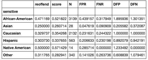
A short explanation about this table follows:
- reoffend: frequencies of reoffending
- score: average score for the group
- N: the total number of people in the group
- FPR: false positive rates
- FNR: false negative rates
- DFP: disproportionate false positive
- DFN: disproportionate false negative
The last FPR and FNR columns together can give an idea about the general quality of the model. If both are high, the model just doesn't perform well for the particular group. The last two columns express the adverse impact ratio of FPR and FNR ratios, respectively, which is what we'll mostly focus on. We need to reduce the racial bias in the model by reducing the FPR of African-Americans to a tolerable level.
Let's do some preprocessing and then we'll build the model:
from sklearn.feature_extraction.text import CountVectorizer
from category_encoders.one_hot import OneHotEncoder
from sklearn.model_selection import train_test_split
from sklearn.preprocessing import StandardScaler

charge_desc = data['c_charge_desc'].apply(lambda x: x if isinstance(x, str) else '')
count_vectorizer = CountVectorizer(
    max_df=0.85, stop_words='english',
    max_features=100, decode_error='ignore'
)
charge_desc_features = count_vectorizer.fit_transform(charge_desc)

one_hot_encoder = OneHotEncoder()
charge_degree_features = one_hot_encoder.fit_transform(
    data['c_charge_degree']
)

data['race_black'] = data['race'].apply(lambda x: x == 'African-American').astype(int)
stratification = data['race_black'] + (data['is_recid']).astype(int) * 2
CountVectorizer counts a vocabulary of words, indicating how many times each word is used. This is called a bag-of-words representation, and we apply it to the charge description column. We exclude English stop words, which are very common words such as prepositions (such as on or at) and personal pronouns (for example I or me); we also limit the vocabulary to 100 words and words that don't appear in more than 85% of the fields.
We apply dummy encoding (one-hot encoding) to the charge degree.
Why do we use two different transformations? Basically, the description is a textual description of why someone was charged with a crime. Every field is different. If we used one-hot encoding, every field would get their own dummy variable, and we wouldn't be able to see any commonalities between fields.
In the end, we create a new variable for stratification in order to make sure that we have similar proportions in the training and test datasets for both recidivism (our target variable) and whether someone is African-American. This will help us to calculate metrics to check for discrimination:
y = data['is_recid']
X = pd.DataFrame(
    data=np.column_stack(
        [data[['juv_fel_count', 'juv_misd_count',
 'juv_other_count', 'priors_count', 'days_b_screening_arrest']],
          charge_degree_features,
          charge_desc_features.todense()
        ]
    ),
    columns=['juv_fel_count', 'juv_misd_count', 'juv_other_count', 'priors_count', 'days_b_screening_arrest'] \
    + one_hot_encoder.get_feature_names() \
    + count_vectorizer.get_feature_names(),
    index=data.index
)
X['jailed_days'] = (data['c_jail_out'] - data['c_jail_in']).apply(lambda x: abs(x.days))
X['waiting_jail_days'] = (data['c_jail_in'] - data['c_offense_date']).apply(lambda x: abs(x.days))
X['waiting_arrest_days'] = (data['c_arrest_date'] - data['c_offense_date']).apply(lambda x: abs(x.days))
X.fillna(0, inplace=True)


columns = list(X.columns)
X_train, X_test, y_train, y_test = train_test_split(
    X, y, test_size=0.33,
    random_state=42,
    stratify=stratification
)  # we stratify by black and the target
We do some data engineering, deriving variables to record how many days someone has spent in jail, has waited for a trial, or has waited for an arrest.
We'll build a neural network model using jax similar to the one we've encountered in the Classifying in scikit-learn, Keras, and PyTorch recipe in Chapter 1, Getting Started with Artificial Intelligence in Python. This time, we'll do a fully fledged implementation:
import jax.numpy as jnp
from jax import grad, jit, vmap, ops, lax
import numpy.random as npr
import numpy as onp
import random
from tqdm import trange
from sklearn.base import ClassifierMixin
from sklearn.preprocessing import StandardScaler


class JAXLearner(ClassifierMixin):
  def __init__(self, layer_sizes=[10, 5, 1], epochs=20, batch_size=500, lr=1e-2):
    self.params = self.construct_network(layer_sizes)
    self.perex_grads = jit(grad(self.error))
    self.epochs = epochs
    self.batch_size = batch_size
    self.lr = lr

  @staticmethod
  def construct_network(layer_sizes=[10, 5, 1]):
    '''Please make sure your final layer corresponds to targets in dimensions.
    '''
    def init_layer(n_in, n_out):
      W = npr.randn(n_in, n_out)
      b = npr.randn(n_out,)
      return W, b

    return list(map(init_layer, layer_sizes[:-1], layer_sizes[1:]))

  @staticmethod
  def sigmoid(X):  # or tanh
    return 1/(1+jnp.exp(-X))

  def _predict(self, inputs):
    for W, b in self.params:
      outputs = jnp.dot(inputs, W) + b
      inputs = self.sigmoid(outputs)
    return outputs

  def predict(self, inputs):
    inputs = self.standard_scaler.transform(inputs)
    return onp.asarray(self._predict(inputs))

  @staticmethod
  def mse(preds, targets, other=None):
    return jnp.sqrt(jnp.sum((preds - targets)**2))

  @staticmethod
  def penalized_mse(preds, targets, sensitive):
    err = jnp.sum((preds - targets)**2)
    err_s = jnp.sum((preds * sensitive - targets * sensitive)**2)
    penalty = jnp.clip(err_s / err, 1.0, 2.0)
    return err * penalty

  def error(self, params, inputs, targets, sensitive):
      preds = self._predict(inputs)
      return self.penalized_mse(preds, targets, sensitive)

  def fit(self, X, y, sensitive):
    self.standard_scaler = StandardScaler()
    X = self.standard_scaler.fit_transform(X)
    N = X.shape[0]
    indexes = list(range(N))
    steps_per_epoch = N // self.batch_size

    for epoch in trange(self.epochs, desc='training'):
        random.shuffle(indexes)
        index_offset = 0
        for step in trange(steps_per_epoch, desc='iteration'):
            grads = self.perex_grads(
                self.params,
                X[indexes[index_offset:index_offset+self.batch_size], :],
                y[indexes[index_offset:index_offset+self.batch_size]],
                sensitive[indexes[index_offset:index_offset+self.batch_size]]
            )
            # print(grads)
            self.params = [(W - self.lr * dW, b - self.lr * db)
                      for (W, b), (dW, db) in zip(self.params, grads)]
            index_offset += self.batch_size
This is a scikit-learn wrapper of a JAX neural network. For scikit-learn compatibility, we inherit from ClassifierMixin and implement fit() and predict(). The most important part here is the penalized MSE method, which, in addition to model predictions and targets, takes into account a sensitive variable.
Let's train it and check the performance. Please note that we feed in X, y, and sensitive_train, which we define as the indicator variable for African-American for the training dataset:
sensitive_train = X_train.join(
    data, rsuffix='_right'
)['race_black']
jax_learner = JAXLearner([X.values.shape[1], 100, 1])
jax_learner.fit(
    X_train.values,
    y_train.values,
    sensitive_train.values
)
We visualize the statistics as follows:
X_predicted = pd.DataFrame(
    data=jax_learner.predict(
        X_test.values
    ) * 10,
    columns=['score'],
    index=X_test.index
).join(
    data[['sex', 'race', 'is_recid']],
    rsuffix='_right'
)
calculate_impacts(X_predicted, score_col='score')
This is the table we get:
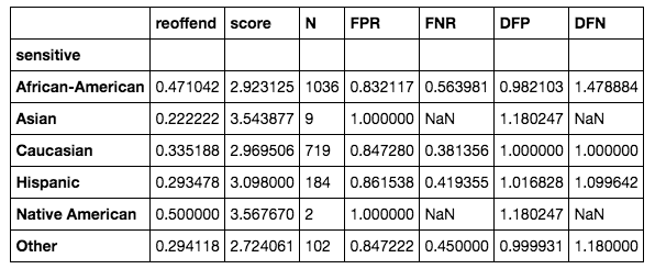
We can see that the disproportionate false positive rate for African-Americans is very close to (and even lower than) 1.0, which is what we wanted. The test set is small and doesn't contain enough samples for Asians and native Americans, so we can't calculate meaningful statistics for those groups. We could, however, extend our approach to encompass these two groups as well if we wanted to ensure that these two groups had equal false positive rates.
How it works...
The keys for this to work are custom objective functions or loss functions. This is far from straightforward in scikit-learn, although we will show an implementation in the following section.
Generally, there are different possibilities for implementing your own cost or loss functions.
- LightGBM, Catboost, and XGBoost each provide an interface with many loss functions and the ability to define custom loss functions.
- PyTorch and Keras (TensorFlow) provide an interface.
- You can implement your model from scratch (this is what we've done in the main recipe).
Scikit-learn generally does not provide a public API for defining your own loss functions. For many algorithms, there is only a single choice, and sometimes there are a couple of alternatives. The rationale in the case of split criteria with trees is that loss functions have to be performant, and only Cython implementations will guarantee this. This is only available in a non-public API, which means it is more difficult to use.
Finally, when there's no (straightforward) way to implement a custom loss, you can wrap your algorithms in a general optimization scheme such as genetic algorithms.
In neural networks, as long as you provide a differentiable loss function, you can plug in anything you want.
Basically, we were able to encode the adverse impact as a penalty term with the Mean Squared Error (MSE) function. It is based on the MSE that we've mentioned before, but has a penalty term for adverse impact. Let's look again at the loss function:
  @staticmethod
  def penalized_mse(preds, targets, sensitive):
    err = jnp.sum((preds - targets)**2)
    err_s = jnp.sum((preds * sensitive - targets * sensitive)**2)
    penalty = jnp.clip(err_s / err, 1.0, 2.0)
    return err * penalty
The first thing to note is that instead of two variables, we pass three variables. sensitive is the variable relevant to the adverse impact, indicating if we have a person from a protected group.
The calculation works as follows:
- We calculate the MSE overall, err, from model predictions and targets.
- We calculate the MSE for the protected group, err_s.
- We take the ratio of the MSE for the protected group over the MSE overall (AIR) and limit it to between 1.0 and 2.0. We don't want values lower than 1, because we are only interested in the AIR if it's negatively affecting the protected group.
- We then multiply AIR by the overall MSE.
As for 2, the MSE can simply be calculated by multiplying the predictions and targets, each by sensitive. That would cancel out all points, where sensitive is equal to 0.
As for 4, it might seem that this would cancel out the overall error, but we see that it actually seems to work. We probably could have added the two terms as well to give both errors a similar importance.
We use the autograd functionality in Jax to differentiate this.
There's more...
In the following, we'll use the non-public scikit-learn API to implement a custom split criterion for decision trees. We'll use this to train a random forest model with the COMPAS dataset:
%%cython

from sklearn.tree._criterion cimport ClassificationCriterion
from sklearn.tree._criterion cimport SIZE_t

import numpy as np
cdef double INFINITY = np.inf

from libc.math cimport sqrt, pow
from libc.math cimport abs


cdef class PenalizedHellingerDistanceCriterion(ClassificationCriterion):

    cdef double proxy_impurity_improvement(self) nogil:
        cdef double impurity_left
        cdef double impurity_right

        self.children_impurity(&impurity_left, &impurity_right)

        return impurity_right + impurity_left

    cdef double impurity_improvement(self, double impurity) nogil:
        cdef double impurity_left
        cdef double impurity_right

        self.children_impurity(&impurity_left, &impurity_right)
        return impurity_right + impurity_left

    cdef double node_impurity(self) nogil:
        cdef SIZE_t* n_classes = self.n_classes
        cdef double* sum_total = self.sum_total
        cdef double hellinger = 0.0
        cdef double sq_count
        cdef double count_k
        cdef SIZE_t k
        cdef SIZE_t c

        for k in range(self.n_outputs):
            for c in range(n_classes[k]):
                hellinger += 1.0

        return hellinger / self.n_outputs

    cdef void children_impurity(self, double* impurity_left,
                                double* impurity_right) nogil:
        cdef SIZE_t* n_classes = self.n_classes
        cdef double* sum_left = self.sum_left
        cdef double* sum_right = self.sum_right
        cdef double hellinger_left = 0.0
        cdef double hellinger_right = 0.0
        cdef double count_k1 = 0.0
        cdef double count_k2 = 0.0

        cdef SIZE_t k
        cdef SIZE_t c

        # stop splitting in case reached pure node with 0 samples of second class
        if sum_left[1] + sum_right[1] == 0:
            impurity_left[0] = -INFINITY
            impurity_right[0] = -INFINITY
            return

        for k in range(self.n_outputs):
            if(sum_left[0] + sum_right[0] > 0):
                count_k1 = sqrt(sum_left[0] / (sum_left[0] + sum_right[0]))
            if(sum_left[1] + sum_right[1] > 0):
                count_k2 = sqrt(sum_left[1] / (sum_left[1] + sum_right[1]))

            hellinger_left += pow((count_k1  - count_k2), 2)

            if(sum_left[0] + sum_right[0] > 0):
                count_k1 = sqrt(sum_right[0] / (sum_left[0] + sum_right[0]))
            if(sum_left[1] + sum_right[1] > 0):
                count_k2 = sqrt(sum_right[1] / (sum_left[1] + sum_right[1]))

            if k==0:
              hellinger_right += pow((count_k1  - count_k2), 2)
            else:
              hellinger_right -= pow((count_k1  - count_k2), 2)

        impurity_left[0]  = hellinger_left  / self.n_outputs
        impurity_right[0] = hellinger_right / self.n_outputs
Let's use this for training and test it:
ensemble = [
    DecisionTreeClassifier(
      criterion=PenalizedHellingerDistanceCriterion(
        2, np.array([2, 2], dtype='int64')
      ),
      max_depth=100
    ) for i in range(100)
]
for model in ensemble:
    model.fit(
        X_train,
        X_train.join(
            data,
            rsuffix='_right'
        )[['is_recid', 'race_black']]
    )
Y_pred = np.array(
    [model.predict(X_test) for model in
     ensemble]
)
predictions2 = Y_pred.mean(axis=0)
This gives us an AUC of 0.62:
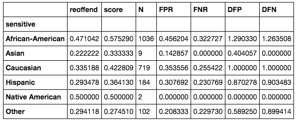
We can see that, although we came a long way, we didn't completely remove all bias. 30% (DFP for African-Americans) would still be considered unacceptable. We could try different refinements or sampling strategies to improve the result. Unfortunately, we wouldn't be able to use this model in practice.
As an example, a way to address this is to do model selection within the random forest. Since each of the trees would have their own way of classifying people, we could calculate the adverse impact statistics for each of the individual trees or combinations of trees. We could remove trees until we are left with a subset of trees that satisfy our adverse impact conditions. This is beyond the scope of this chapter.
See also
You can read up more on algorithmic fairness in different places. There's a wide variety of literature available on fairness:
- A Science Magazine article about the COMPAS model (Julia Dressel and Hany Farid, 2018, The accuracy, fairness, and limits of predicting recidivism): https://advances.sciencemag.org/content/4/1/eaao5580
- A comparative study of fairness-enhancing interventions in machine learning (Sorelle Friedler and others, 2018): https://arxiv.org/pdf/1802.04422.pdf
- A Survey on Bias and Fairness in Machine Learning (Mehrabi and others, 2019): https://arxiv.org/pdf/1908.09635.pdf
- The effect of explaining fairness (Jonathan Dodge and others, 2019): https://arxiv.org/pdf/1901.07694.pdf
Different Python libraries are available for tackling bias (or, inversely, algorithmic fairness):
- fairlearn: https://github.com/fairlearn/fairlearn
- AIF360: https://github.com/IBM/AIF360
- FairML: https://github.com/adebayoj/fairml
- BlackBoxAuditing: https://github.com/algofairness/BlackBoxAuditing
- Balanced Committee Election: https://github.com/huanglx12/Balanced-Committee-Election
Finally, Scikit-Lego includes functionality for fairness: https://scikit-lego.readthedocs.io/en/latest/fairness.html
While you can find many datasets on recidivism by performing a Google dataset search (https://toolbox.google.com/datasetsearch), there are many more applications and corresponding datasets where fairness is important, such as credit scoring, face recognition, recruitment, or predictive policing, to name just a few.
There are different places to find out more about custom losses. The article Custom loss versus custom scoring (https://kiwidamien.github.io/custom-loss-vs-custom-scoring.html) affords a good overview. For implementations of custom loss functions in gradient boosting, towardsdatascience (https://towardsdatascience.com/custom-loss-functions-for-gradient-boosting-f79c1b40466d) is a good place to start.


