It's a good idea to double-check our installation. While our terminal is still open, we fire up IPython, which is an interactive shell to run Python commands:
$ ipython
Now make sure that you are running (at least) Python 3.5 and not Python 2.7. You might see the version number displayed in IPython's welcome message. If not, you can run the following commands:
In [1]: import sys
...     print(sys.version)
        3.5.3 |Continuum Analytics, Inc.| (default, Feb 22 2017,   21:28:42) [MSC v.1900 64 bit (AMD64)]
Now try to import OpenCV:
In [2]: import cv2
You should get no error messages. Then, try to find out the version number:
In [3]: cv2.__version__
Out[3]: '3.1.0'
Make sure that the Python version reads 3.5 or 3.6, but not 2.7. Additionally, make sure that OpenCV's version number reads at least 3.1.0; otherwise, you will not be able to use some OpenCV functionality later on.
OpenCV 3 is actually called cv2. I know it's confusing. Apparently, the reason for this is that the 2 does not stand for the version number. Instead, it is meant to highlight the difference between the underlying C API (which is denoted by the cv prefix) and the C++ API (which is denoted by the cv2 prefix).
You can then exit the IPython shell by typing exit - or hitting Ctrl + D and confirming that you want to quit.
Alternatively, you can run the code in a web browser thanks to Jupyter Notebook. If you have never heard of Jupyter Notebooks or played with them before, trust me - you will love them! If you followed the directions as mentioned earlier and installed the Python Anaconda stack, Jupyter is already installed and ready to go. In a terminal, type as follows:
$ jupyter notebook
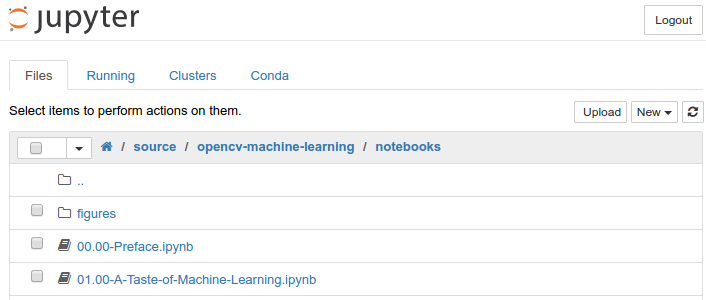
This will automatically open a browser window, showing a list of files in the current directory. Click on the opencv-machine-learning folder, then on the notebooks folder, and voila! Here you will find all the code for this book, ready for you to be explored:
Beginning of the list of Jupyter Notebooks that come with this book
The notebooks are arranged by chapter and section. For the most part, they contain only the relevant code, but no additional information or explanations. These are reserved for those who support our effort by buying this book - so thank you!
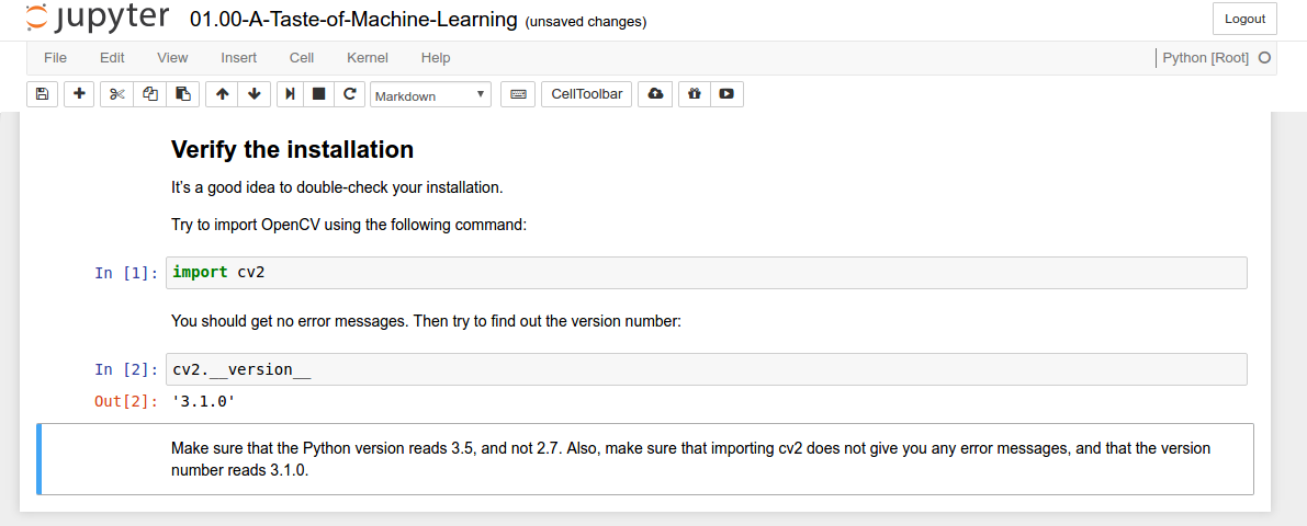
Simply click on a notebook of your choice, such as 01.00-A-Taste-of-Machine-Learning.ipynb, and you will be able to run the code yourself by selecting Kernel > Restart & Run All:
Example excerpt of this chapter's Jupyter Notebook
There are a few handy keyboard shortcuts for navigating Jupyter Notebooks. However, the only ones that you need to know about right now are the following:
- Click in a cell in order to edit it.
- While the cell is selected, hit Ctrl + Enter to execute the code in it.
- Alternatively, hit Shift + Enter to execute a cell and select the cell below it.
- Hit Esc to exit write mode, then hit A to insert a cell above the currently selected one and B to insert a cell below.
Check out all the keyboard shortcuts by clicking on Help > Keyboard Shortcut, or take a quick tour by clicking on Help > User Interface Tour.
However, I strongly encourage you to follow along the book by actually typing out the commands yourself, preferably in an IPython shell or an empty Jupyter Notebook. There is no better way to learn how to code than by getting your hands dirty. Even better if you make mistakes--we have all been there. At the end of the day, it's all about learning by doing!


