Predicting classification
You learned that XGBoost may have an edge in regression, but what about classification? XGBoost has a classification model, but will it perform as accurately as well tested classification models such as logistic regression? Let's find out.
What is classification?
Unlike with regression, when predicting target columns with a limited number of outputs, a machine learning algorithm is categorized as a classification algorithm. The possible outputs may include the following:
Yes, No
Spam, Not Spam
0, 1
Red, Blue, Green, Yellow, Orange
Dataset 2 – The census
We will move a little more swiftly through the second dataset, the Census Income Data Set (https://archive.ics.uci.edu/ml/datasets/Census+Income), to predict personal income.
Data wrangling
Before implementing machine learning, the dataset must be preprocessed. When testing new algorithms, it's essential to have all numerical columns with no null values.
Data loading
Since this dataset is hosted directly on the UCI Machine Learning website, it can be downloaded directly from the internet using pd.read_csv:
df_census = pd.read_csv('https://archive.ics.uci.edu/ml/machine-learning-databases/adult/adult.data')
df_census.head()
Here is the expected output:
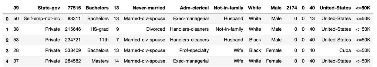
Figure 1.12 – The Census Income DataFrame
The output reveals that the column headings represent the entries of the first row. When this happens, the data may be reloaded with the header=None parameter:
df_census = pd.read_csv('https://archive.ics.uci.edu/ml/machine-learning-databases/adult/adult.data', header=None)
df_census.head()
Here is the expected output without the header:
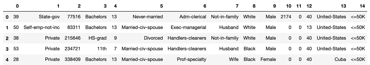
Figure 1.13 – The header=None parameter output
As you can see, the column names are still missing. They are listed on the Census Income Data Set website (https://archive.ics.uci.edu/ml/datasets/Census+Income) under Attribute Information.
Column names may be changed as follows:
df_census.columns=['age', 'workclass', 'fnlwgt', 'education', 'education-num', 'marital-status', 'occupation', 'relationship', 'race', 'sex', 'capital-gain', 'capital-loss', 'hours-per-week', 'native-country', 'income']
df_census.head()
Here is the expected output with column names:
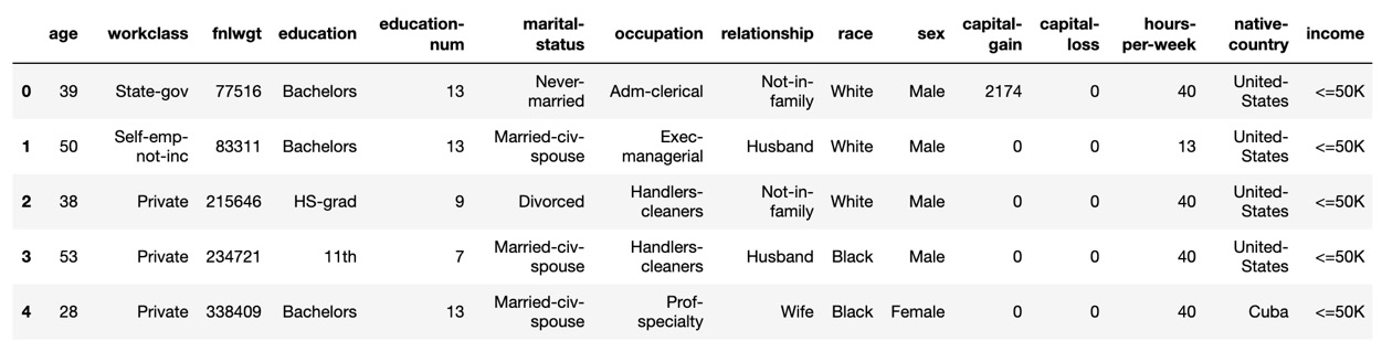
Figure 1.14 – Expected column names
As you can see, the column names have been restored.
Null values
A great way to check null values is to look at the DataFrame .info() method:
df_census.info()
The output is as follows:
<class 'pandas.core.frame.DataFrame'>
RangeIndex: 32561 entries, 0 to 32560
Data columns (total 15 columns):
 #   Column          Non-Null Count  Dtype
---  ------          --------------  -----
 0   age             32561 non-null  int64
 1   workclass       32561 non-null  object
 2   fnlwgt          32561 non-null  int64
 3   education       32561 non-null  object
 4   education-num   32561 non-null  int64
 5   marital-status  32561 non-null  object
 6   occupation      32561 non-null  object
 7   relationship    32561 non-null  object
 8   race            32561 non-null  object
 9   sex             32561 non-null  object
 10  capital-gain    32561 non-null  int64
 11  capital-loss    32561 non-null  int64
 12  hours-per-week  32561 non-null  int64
 13  native-country  32561 non-null  object
 14  income          32561 non-null  object
dtypes: int64(6), object(9)
memory usage: 3.7+ MB
Since all columns have the same number of non-null rows, we can infer that there are no null values.
Non-numerical columns
All columns of the dtype object must be transformed into numerical columns. A pandas get_dummies method takes the non-numerical unique values of every column and converts them into their own column, with 1 indicating presence and 0 indicating absence. For instance, if the column values of a DataFrame called "Book Types" were "hardback," "paperback," or "ebook," pd.get_dummies would create three new columns called "hardback," "paperback," and "ebook" replacing the "Book Types" column.
Here is a "Book Types" DataFrame:
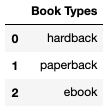
Figure 1.15 – A "Book Types" DataFrame
Here is the same DataFrame after pd.get_dummies:
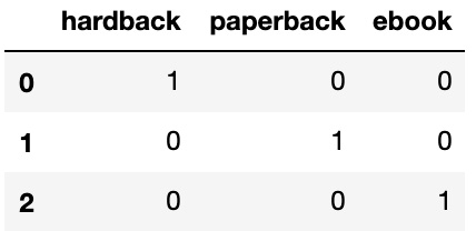
Figure 1.16 – The new DataFrame
pd.get_dummies will create many new columns, so it's worth checking to see whether any columns may be eliminated. A quick review of the df_census data reveals an 'education' column and an education_num column. The education_num column is a numerical conversion of 'education'. Since the information is the same, the 'education' column may be deleted:
df_census = df_census.drop(['education'], axis=1)
Now use pd.get_dummies to transform the non-numerical columns into numerical columns:
df_census = pd.get_dummies(df_census)
df_census.head()
Here is the expected output:
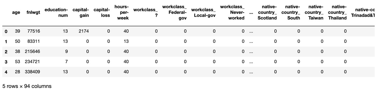
Figure 1.17 – pd.get_dummies – non-numerical to numerical columns
As you can see, new columns are created using a column_value syntax referencing the original column. For example, native-country is an original column, and Taiwan is one of many values. The new native-country_Taiwan column has a value of 1 if the person is from Taiwan and 0 otherwise.
Tip
Using pd.get_dummies may increase memory usage, as can be verified using the .info() method on the DataFrame in question and checking the last line. Sparse matrices may be used to save memory where only values of 1 are stored and values of 0 are not stored. For more information on sparse matrices, see Chapter 10, XGBoost Model Deployment, or visit SciPy's official documentation at https://docs.scipy.org/doc/scipy/reference/.
Target and predictor columns
Since all columns are numerical with no null values, it's time to split the data into target and predictor columns.
The target column is whether or not someone makes 50K. After pd.get_dummies, two columns, df_census['income_<=50K'] and df_census['income_>50K'], are used to determine whether someone makes 50K. Since either column will work, we delete df_census['income_ <=50K']:
df_census = df_census.drop('income_ <=50K', axis=1)
Now split the data into X (predictor columns) and y (target column). Note that -1 is used for indexing since the last column is the target column:
X = df_census.iloc[:,:-1]y = df_census.iloc[:,-1]
It's time to build machine learning classifiers!
Logistic regression
Logistic regression is the most fundamental classification algorithm. Mathematically, logistic regression works in a manner similar to linear regression. For each column, logistic regression finds an appropriate weight, or coefficient, that maximizes model accuracy. The primary difference is that instead of summing each term, as in linear regression, logistic regression uses the sigmoid function.
Here is the sigmoid function and the corresponding graph:
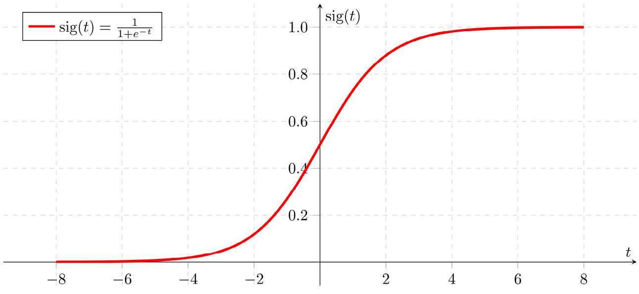
Figure 1.18 – Sigmoid function graph
The sigmoid is commonly used for classification. All values greater than 0.5 are matched to 1, and all values less than 0.5 are matched to 0.
Implementing logistic regression with scikit-learn is nearly the same as implementing linear regression. The main differences are that the predictor column should fit into categories, and the error should be in terms of accuracy. As a bonus, the error is in terms of accuracy by default, so explicit scoring parameters are not required.
You may import logistic regression as follows:
from sklearn.linear_model import LogisticRegression
The cross-validation function
Let's use cross-validation on logistic regression to predict whether someone makes over 50K.
Instead of copying and pasting, let's build a cross-validation classification function that takes a machine learning algorithm as input and has the accuracy score as output using cross_val_score:
def cross_val(classifier, num_splits=10): model = classifier scores = cross_val_score(model, X, y, cv=num_splits) print('Accuracy:', np.round(scores, 2)) print('Accuracy mean: %0.2f' % (scores.mean()))
Now call the function with logistic regression:
cross_val(LogisticRegression())
The output is as follows:
Accuracy: [0.8  0.8  0.79 0.8  0.79 0.81 0.79 0.79 0.8  0.8 ]
Accuracy mean: 0.80
80% accuracy isn't bad out of the box.
Let's see whether XGBoost can do better.
Tip
Any time you find yourself copying and pasting code, look for a better way! One aim of computer science is to avoid repetition. Writing your own data analysis and machine learning functions will make your life easier and your work more efficient in the long run.
The XGBoost classifier
XGBoost has a regressor and a classifier. To use the classifier, import the following algorithm:
from xgboost import XGBClassifier
Now run the classifier in the cross_val function with one important addition. Since there are 94 columns, and XGBoost is an ensemble method, meaning that it combines many models for each run, each of which includes 10 splits, we are going to limit n_estimators, the number of models, to 5. Normally, XGBoost is very fast. In fact, it has a reputation for being the fastest boosting ensemble method out there, a reputation that we will check in this book! For our initial purposes, however, 5 estimators, though not as robust as the default of 100, is sufficient. Details on choosing n_estimators will be a focal point of Chapter 4, From Gradient Boosting to XGBoost:
cross_val(XGBClassifier(n_estimators=5))
The output is as follows:
Accuracy: [0.85 0.86 0.87 0.85 0.86 0.86 0.86 0.87 0.86 0.86]
Accuracy mean: 0.86
As you can see, XGBoost scores higher than logistic regression out of the box.