Understanding the dataset
Here, we are going to discuss our input dataset in order to develop the application. You can find the dataset at https://github.com/jalajthanaki/credit-risk-modelling/tree/master/data.
Let's discuss the dataset and its attributes in detail. Here, in the dataset, you can find the following files:
cs-training.csvRecords in this file are used for training, so this is our training dataset.
cs-test.csvRecords in this file are used for testing our machine learning models, so this is our testing dataset.
Data Dictionary.xlsThis file contains information about each of the attributes of the dataset. So, this file is referred to as our data dictionary.
sampleEntry.csvThis file gives us an idea about the format in which we need to generate our end output for our testing dataset. If you open this file, then you will see that we need to generate the probability of each of the records present in the testing dataset. This probability value indicates the chances of borrowers defaulting.
Understanding attributes of the dataset
The dataset has 11 attributes, which are shown as follows:

Figure 1.1: Attributes (variables) of the dataset
We will look at each of the attributes one by one and understand their meaning in the context of the application:
SeriousDlqin2yrs:
In the dataset, this particular attribute indicates whether the borrower has experienced any past dues until 90 days in the previous 2 years.
The value of this attribute is Yes if the borrower has experienced past dues of more than 90 days in the previous 2 years. If the EMI was not paid by the borrower 90 days after the due date of the EMI, then this flag value is Yes.
The value of this attribute is No if the borrower has not experienced past dues of more than 90 days in the previous 2 years. If the EMI was paid by the borrower before 90 days from the due date of the EMI, then this flag value is No.
This attribute has target labels. In other words, we are going to predict this value using our algorithm for the test dataset.
RevolvingUtilizationOfUnsecuredLines:
This attribute indicates the credit card limits of the borrower after excluding any current loan debt and real estate.
Suppose I have a credit card and its credit limit is $1,000. In my personal bank account, I have $1,000. My credit card balance is $500 out of $1,000.
So, the total maximum balance I can have via my credit card and personal bank account is $1,000 + $1,000 = $2,000; I have used $500 from my credit card limit, so the total balance that I have is $500 (credit card balance) + $1,000 (personal bank account balance) = $1,500.
If account holder have taken home loan or other property loan and paying EMIs for those loan then we are not considering EMI value for property loan. Here, for this data attribute we have considered account holder's credit card balance and personal account balance.
So, the RevolvingUtilizationOfUnsecuredLines value is = $1,500 / $2,000 = 0.7500
Age:
This attribute is self-explanatory. It indicates the borrower's age.
NumberOfTime30-59DaysPastDueNotWorse:
The number of this attribute indicates the number of times borrowers have paid their EMIs late but have paid them 30 days after the due date or 59 days before the due date.
DebtRatio:
This is also a self-explanatory attribute, but we will try and understand it better with an example.
If my monthly debt is $200 and my other expenditure is $500, then I spend $700 monthly. If my monthly income is $1,000, then the value of the DebtRatio is $700/$1,000 = 0.7000
MonthlyIncome:
This attribute contains the value of the monthly income of borrowers.
NumberOfOpenCreditLinesAndLoans:
This attribute indicates the number of open loans and/or the number of credit cards the borrower holds.
NumberOfTimes90DaysLate:
This attribute indicates how many times a borrower has paid their dues 90 days after the due date of their EMIs.
NumberRealEstateLoansOrLines:
This attribute indicates the number of loans the borrower holds for their real estate or the number of home loans a borrower has.
NumberOfTime60-89DaysPastDueNotWorse:
This attribute indicates how many times borrowers have paid their EMIs late but paid them 60 days after their due date or 89 days before their due date.
NumberOfDependents:
This attribute is self-explanatory as well. It indicates the number of dependent family members the borrowers have. The dependent count is excluding the borrower.
These are basic attribute descriptions of the dataset, so you have a basic idea of the kind of dataset we have. Now it's time to get hands-on. So from the next section onward, we will start coding. We will begin exploring our dataset by performing basic data analysis so that we can find out the statistical properties of the dataset.
Data analysis
This section is divided into two major parts. You can refer to the following figure to see how we will approach this section:
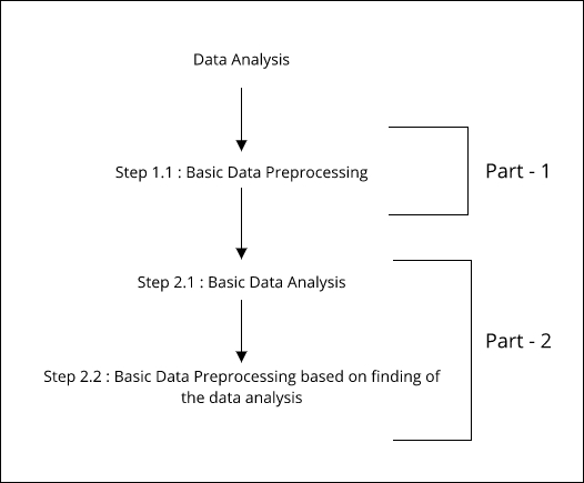
Figure 1.2: Parts and steps of data analysis
In the first part, we have only one step. In the preceding figure, this is referred to as step 1.1. In this first step, we will do basic data preprocessing. Once we are done with that, we will start with our next part.
The second part has two steps. In the figure, this is referred to as step 2.1. In this step, we will perform basic data analysis using statistical and visualization techniques, which will help us understand the data. By doing this activity, we will get to know some statistical facts about our dataset. After this, we will jump to the next step, which is referred to as step 2.2 in Figure 1.2. In this step, we will once again perform data preprocessing, but, this time, our preprocessing will be heavily based on the findings that we have derived after doing basic data analysis on the given training dataset. You can find the code at this GitHub Link: https://github.com/jalajthanaki/credit-risk-modelling/blob/master/basic_data_analysis.ipynb.
So let's begin!
Data preprocessing
In this section, we will perform a minimal amount of basic preprocessing. We will look at the approaches as well as their implementation.
First change
If you open the cs-training.csv file, then you will find that there is a column without a heading, so we will add a heading there. Our heading for that attribute is ID. If you want to drop this column, you can because it just contains the sr.no of the records.
Second change
This change is not a mandatory one. If you want to skip it, you can, but I personally like to perform this kind of preprocessing. The change is related to the heading of the attributes, we are removing "-" from the headers. Apart from this, I will convert all the column heading into lowercase. For example, the attribute named NumberOfTime60-89DaysPastDueNotWorse will be converted into numberoftime6089dayspastduenotworse. These kinds of changes will help us when we perform in-depth data analysis. We do not need to take care of this hyphen symbols while processing.
Implementing the changes
Now, you may ask how will I perform the changes described? Well, there are two ways. One is a manual approach. In this approach, you will open the cs-training.csv file and perform the changes manually. This approach certainly isn't great. So, we will take the second approach. With the second approach, we will perform the changes using Python code. You can find all the changes in the following code snippets.
Refer to the following screenshot for the code to perform the first change:
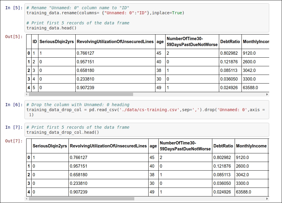
Figure 1.3: Code snippet for implementing the renaming or dropping of the index column
For the second change, you can refer to Figure 1.4:
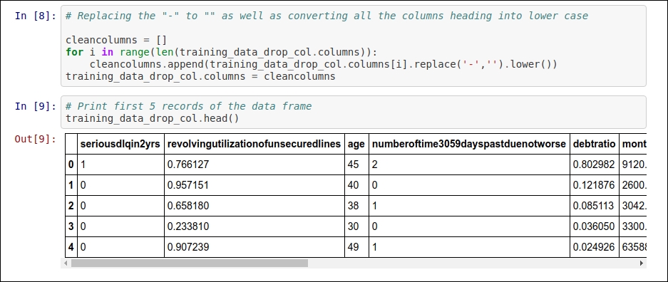
Figure 1.4: Code snippet for removing "-" from the column heading and converting all the column headings into lowercase
The same kind of preprocessing needs to be done on the cs-test.csv file. This is because the given changes are common for both the training and testing datasets.
You can find the entire code on GitHub by clicking on this link: https://github.com/jalajthanaki/credit-risk-modelling/blob/master/basic_data_analysis.ipynb.
You can also move hands-on along with reading.
I'm using Python 2.7 as well as a bunch of different Python libraries for the implementation of this code. You can find information related to Python dependencies as well as installation in the README section. Now let's move on to the basic data analysis section.
Basic data analysis followed by data preprocessing
Let's perform some basic data analysis, which will help us find the statistical properties of the training dataset. This kind of analysis is also called exploratory data analysis (EDA), and it will help us understand how our dataset represents the facts. After deriving some facts, we can use them in order to derive feature engineering. So let's explore some important facts!
From this section onward, all the code is part of one iPython notebook. You can refer to the code using this GitHub Link: https://github.com/jalajthanaki/credit-risk-modelling/blob/master/Credit%20Risk%20Analysis.ipynb.
The following are the steps we are going to perform:
Listing statistical properties
Finding the missing values
Replacing missing values
Correlation
Detecting Outliers
Listing statistical properties
In this section, we will get an idea about the statistical properties of the training dataset. Using pandas' describe function, we can find out the following basic things:
count: This will give us an idea about the number of records in our training dataset.mean: This value gives us an indication of the mean of each of the data attributes.std: This value indicates the standard deviation for each of the data attributes. You can refer to this example: http://www.mathsisfun.com/data/standard-deviation.html.min: This value gives us an idea of what the minimum value for each of the data attributes is.25%: This value indicates the 25th percentile. It should fall between 0 and 1.50%: This value indicates the 50th percentile. It should fall between 0 and 1.75%: This value indicates the 75th percentile. It should fall between 0 and 1.max: This value gives us an idea of what the maximum value for each of the data attributes is.
Take a look at the code snippet in the following figure:

Figure 1.5: Basic statistical properties using the describe function of pandas
We need to find some other statistical properties for our dataset that will help us understand it. So, here, we are going to find the median and mean for each of the data attributes. You can see the code for finding the median in the following figure:
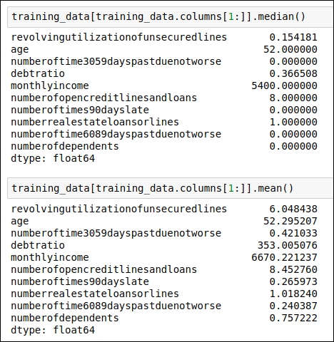
Figure 1.6: Code snippet for generating the median and the mean for each data attribute
Now let's check out what kind of data distribution is present in our dataset. We draw the frequency distribution for our target attribute, seriousdlqin2yrs, in order to understand the overall distribution of the target variable for the training dataset. Here, we will use the seaborn visualization library. You can refer to the following code snippet:
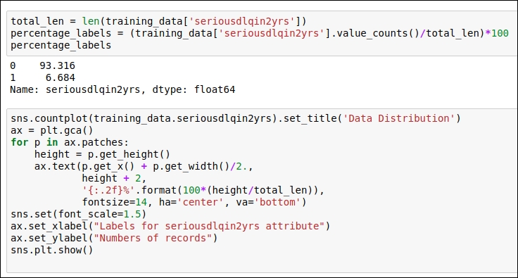
Figure 1.7: Code snippet for understanding the target variable distribution as well as the code snippet for the visualization of the distribution
You can refer to the visualization chart in the following figure:
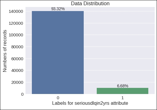
Figure 1.8: Visualization of the variable distribution of the target data attribute
From this chart, you can see that there are many records with the target label 0 and fewer records with the target label 1. You can see that the data records with a 0 label are about 93.32%, whereas 6.68% of the data records are labeled 1. We will use all of these facts in the upcoming sections. For now, we can consider our outcome variable as imbalanced.
Finding missing values
In order to find the missing values in the dataset, we need to check each and every data attribute. First, we will try to identify which attribute has a missing or null value. Once we have found out the name of the data attribute, we will replace the missing value with a more meaningful value. There are a couple of options available for replacing the missing values. We will explore all of these possibilities.
Let's code for our first step. Here, we will see which data attribute has missing values as well count how many records there are for each data attribute with a missing value. You can see the code snippet in the following figure:
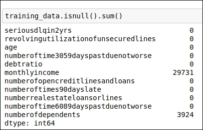
Figure 1.9: Code snippet for identifying which data attributes have missing values
As displayed in the preceding figure, the following two data attributes have missing values:
monthlyincome: This attribute contains 29,731 records with a missing value.numberofdependents: This attribute contains 3,924 records with a missing value.
You can also refer to the code snippet in the following figure for the graphical representation of the facts described so far:
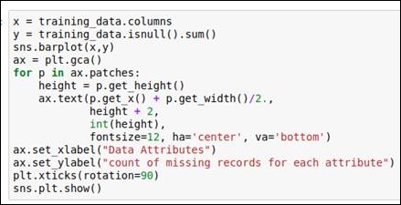
Figure 1.10: Code snippet for generating a graph of missing values
You can view the graph itself in the following figure:
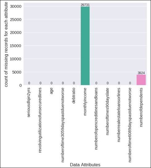
Figure 1.11: A graphical representation of the missing values
In this case, we need to replace these missing values with more meaningful values. There are various standard techniques that we can use for that. We have the following two options:
Replace the missing value with the mean value of that particular data attribute
Replace the missing value with the median value of that particular data attribute
In the previous section, we already derived the mean and median values for all of our data attributes, and we will use them. Here, our focus will be on the attributes titled monthlyincome and numberofdependents because they have missing values. We have found out which data attributes have missing values, so now it's time to perform the actual replacement operation. In the next section, you will see how we can replace the missing values with the mean or the median.
Replacing missing values
In the previous section, we figured out which data attributes in our training dataset contain missing values. We need to replace the missing values with either the mean or the median value of that particular data attribute. So in this section, we will focus particularly on how we can perform the actual replacement operation. This operation of replacing the missing value is also called imputing the missing data.
Before moving on to the code section, I feel you guys might have questions such as these: should I replace missing values with the mean or the median? Are there any other options available? Let me answer these questions one by one.
The answer to the first question, practically, will be a trial and error method. So you first replace missing values with the mean value, and during the training of the model, measure whether you get a good result on the training dataset or not. Then, in the second iteration, we need to try to replace the values with the median and measure whether you get a good result on the training dataset or not.
In order to answer the second question, there are many different imputation techniques available, such as the deletion of records, replacing the values using the KNN method, replacing the values using the most frequent value, and so on. You can select any of these techniques, but you need to train the model and measure the result. Without implementing a technique, you can't really say with certainty that a particular imputation technique will work for the given training dataset. Here, we are talking in terms of the credit-risk domain, so I would not get into the theory much, but just to refresh your concepts, you can refer to the following articles:
We can see the code for replacing the missing values using the attribute's mean value and its median value in the following figure:
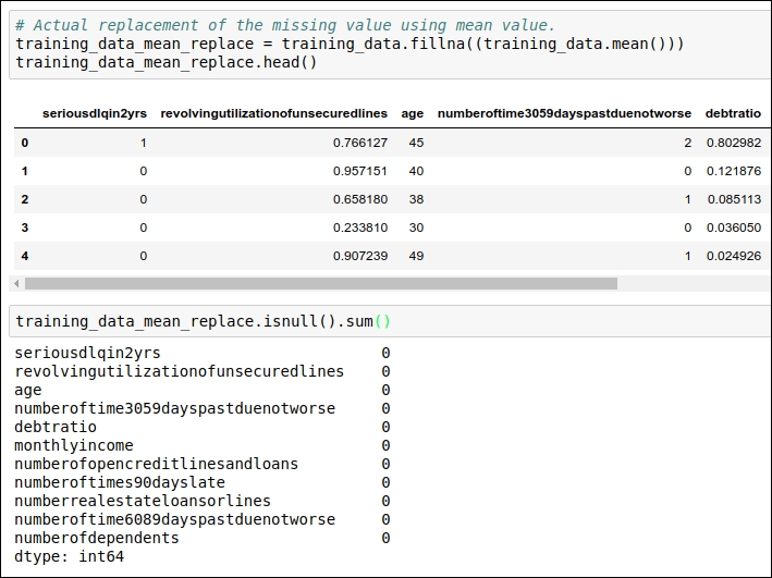
Figure 1.12: Code snippet for replacing the mean values
In the preceding code snippet, we replaced the missing value with the mean value, and in the second step, we verified that all the missing values have been replaced with the mean of that particular data attribute.
In the next code snippet, you can see the code that we have used for replacing the missing values with the median of those data attributes. Refer to the following figure:
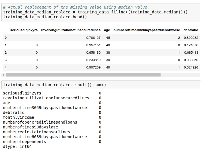
Figure 1.13: Code snippet for replacing missing values with the median
In the preceding code snippet, we have replaced the missing value with the median value, and in second step, we have verified that all the missing values have been replaced with the median of that particular data attribute.
In the first iteration, I would like to replace the missing value with the median.
In the next section, we will see one of the important aspects of basic data analysis: finding correlations between data attributes. So, let's get started with correlation.
Correlation
I hope you basically know what correlation indicates in machine learning. The term correlation refers to a mutual relationship or association between quantities. If you want to refresh the concept on this front, you can refer to https://www.investopedia.com/terms/c/correlation.asp.
So, here, we will find out what kind of association is present among the different data attributes. Some attributes are highly dependent on one or many other attributes. Sometimes, values of a particular attribute increase with respect to its dependent attribute, whereas sometimes values of a particular attribute decrease with respect to its dependent attribute. So, correlation indicates the positive as well as negative associations among data attributes. You can refer to the following code snippet for the correlation:
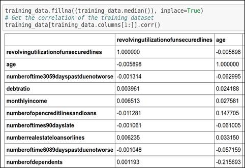
Figure 1.14: Code snippet for generating correlation
You can see the code snippet of the graphical representation of the correlation in the following figure:

Figure 1.15: Code snippet for generating a graphical snippet
You can see the graph of the correlation in the following figure:
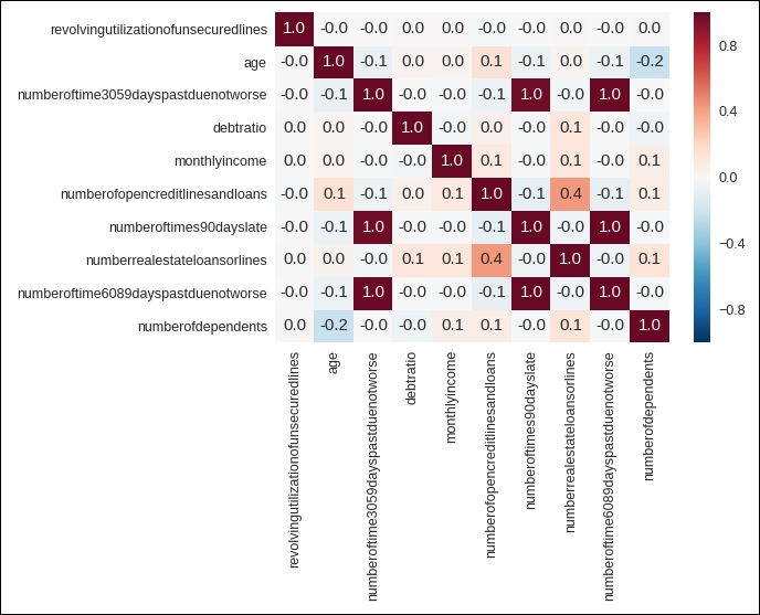
Figure 1.16: Heat map for correlation
Let's look at the preceding graph because it will help you understand correlation in a great way. The following facts can be derived from the graph:
Cells with 1.0 values are highly associated with each other.
Each attribute has a very high correlation with itself, so all the diagonal values are 1.0.
The data attribute numberoftime3059dayspastduenotworse (refer to the data attribute given on the vertical line or on the y axis) is highly associated with two attributes, numberoftimes90dayslate and numberoftime6089dayspastduenotworse. These two data attributes are given on the x axis (or on the horizontal line).
The data attribute numberoftimes90dayslate is highly associated with numberoftime3059dayspastduenotworse and numberoftime6089dayspastduenotworse. These two data attributes are given on the x axis (or on the horizontal line).
The data attribute numberoftime6089dayspastduenotworse is highly associated with numberoftime3059dayspastduenotworse and numberoftimes90dayslate. These two data attributes are given on the x axis (or on the horizontal line).
The data attribute numberofopencreditlinesandloans also has an association with numberrealestateloansorlines and vice versa. Here, the data attribute numberrealestateloansorlines is present on the x axis (or on the horizontal line).
Before moving ahead, we need to check whether these attributes contain any outliers or insignificant values. If they do, we need to handle these outliers, so our next section is about detecting outliers from our training dataset.
Detecting outliers
In this section, you will learn how to detect outliers as well as how to handle them. There are two steps involved in this section:
Outliers detection techniques
Handling outliers
First, let's begin with detecting outliers. Now you guys might have wonder why should we detect outliers. In order to answer this question, I would like to give you an example. Suppose you have the weights of 5-year-old children. You measure the weight of five children and you want to find out the average weight. The children weigh 15, 12, 13, 10, and 35 kg. Now if you try to find out the average of these values, you will see that the answer 17 kg. If you look at the weight range carefully, then you will realize that the last observation is out of the normal range compared to the other observations. Now let's remove the last observation (which has a value of 35) and recalculate the average of the other observations. The new average is 12.5 kg. This new value is much more meaningful in comparison to the last average value. So, the outlier values impact the accuracy greatly; hence, it is important to detect them. Once that is done, we will explore techniques to handle them in upcoming section named handling outlier.
Outliers detection techniques
Here, we are using the following outlier detection techniques:
Percentile-based outlier detection
Median Absolute Deviation (MAD)-based outlier detection
Standard Deviation (STD)-based outlier detection
Majority-vote-based outlier detection
Visualization of outliers
Percentile-based outlier detection
Here, we have used percentile-based outlier detection, which is derived based on the basic statistical understanding. We assume that we should consider all the data points that lie under the percentile range from 2.5 to 97.5. We have derived the percentile range by deciding on a threshold of 95. You can refer to the following code snippet:

Figure 1.17: Code snippet for percentile-based outlier detection
We will use this method for each of the data attributes and detect the outliers.
Median Absolute Deviation (MAD)-based outlier detection
MAD is a really simple statistical concept. There are four steps involved in it. This is also known as modified Z-score. The steps are as follows:
Find the median of the particular data attribute.
For each of the given values for the data attribute, subtract the previously found median value. This subtraction is in the form of the absolute value. So, for each data point, you will get the absolute value.
In the third step, generate the median of the absolute values that we derived in the second step. We will perform this operation for each data point for each of the data attributes. This value is called the MAD value.
In the fourth step, we will use the following equation to derive the modified Z-score:


Now it's time to refer to the following code snippet:

Figure 1.18: Code snippet for MAD-based outlier detection
Standard Deviation (STD)-based outlier detection
In this section, we will use standard deviation and the mean value to find the outlier. Here, we select a random threshold value of 3. You can refer to the following code snippet:
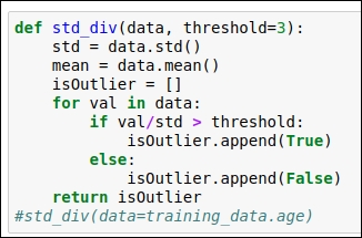
Figure 1.19: Standard Deviation (STD) based outlier detection code
Majority-vote-based outlier detection:
In this section, we will build the voting mechanism so that we can simultaneously run all the previously defined methods—such as percentile-based outlier detection, MAD-based outlier detection, and STD-based outlier detection—and get to know whether the data point should be considered an outlier or not. We have seen three techniques so far. So, if two techniques indicate that the data should be considered an outlier, then we consider that data point as an outlier; otherwise, we don't. So, the minimum number of votes we need here is two. Refer to the following figure for the code snippet:
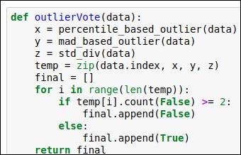
Figure 1.20: Code snippet for the voting mechanism for outlier detection
Visualization of outliers
In this section, we will plot the data attributes to get to know about the outliers visually. Again, we are using the seaborn and matplotlib library to visualize the outliers. You can find the code snippet in the following figure:

Figure 1.21: Code snippet for the visualization of the outliers
Refer to the preceding figure for the graph and learn how our defined methods detect the outlier. Here, we chose a sample size of 5,000. This sample was selected randomly.
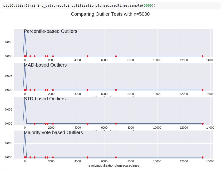
Figure 1.22: Graph for outlier detection
Here, you can see how all the defined techniques will help us detect outlier data points from a particular data attribute. You can see all the attribute visualization graphs on this GitHub link at https://github.com/jalajthanaki/credit-risk-modelling/blob/master/Credit%20Risk%20Analysis.ipynb.
So far, you have learned how to detect outliers, but now it's time to handle these outlier points. In the next section, we will look at how we can handle outliers.
Handling outliers
In this section, you will learn how to remove or replace outlier data points. This particular step is important because if you just identify the outlier but aren't able to handle it properly, then at the time of training, there will be a high chance that we over-fit the model. So, let's learn how to handle the outliers for this dataset. Here, I will explain the operation by looking at the data attributes one by one.
Revolving utilization of unsecured lines
In this data attribute, when you plot an outlier detection graph, you will come to know that values of more than 0.99999 are considered outliers. So, values greater than 0.99999 can be replaced with 0.99999. So for this data attribute, we perform the replacement operation. We have generated new values for the data attribute revolvingutilizationofunsecuredlines.
For the code, you can refer to the following figure:

Figure 1.23: Code snippet for replacing outlier values with 0.99999
Age
In this attribute, if you explore the data and see the percentile-based outlier, then you see that there is an outlier with a value of 0 and the youngest age present in the data attribute is 21. So, we replace the value of 0 with 22. We code the condition such that the age should be more than 22. If it is not, then we will replace the age with 22. You can refer to the following code and graph.
The following figure shows how the frequency distribution of age is given in the dataset. By looking at the data, we can derive the fact that 0 is the outlier value:
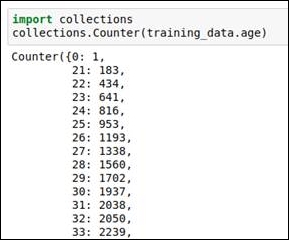
Figure 1.24: Frequency for each data value shows that 0 is an outlier
Refer to the following box graph, which gives us the distribution indication of the age:
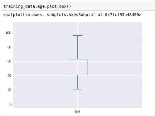
Figure 1.25: Box graph for the age data attribute
Before removing the outlier, we got the following outlier detection graph:
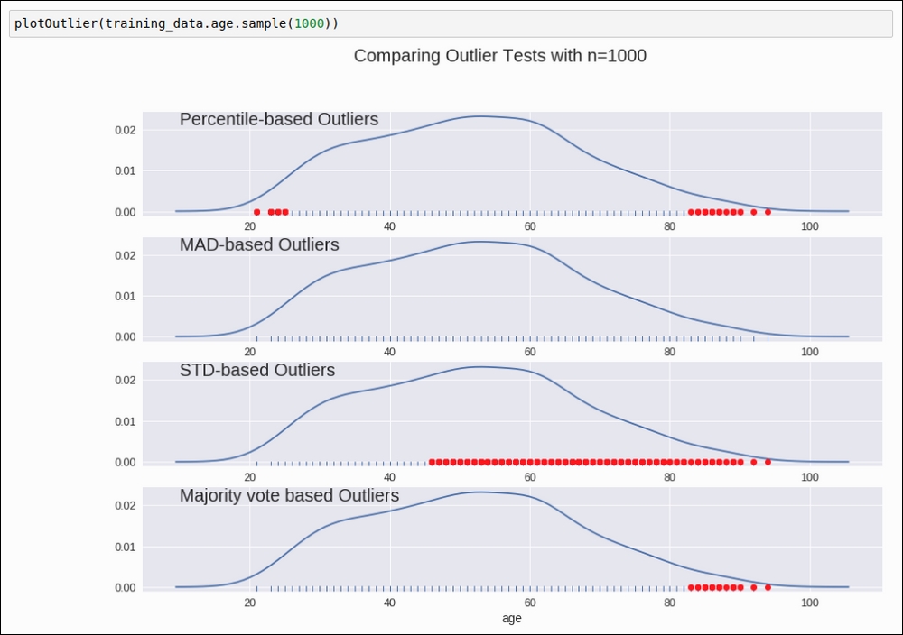
Figure 1.26: Graphical representation of detecting outliers for data attribute age
The code for replacing the outlier is as follows:
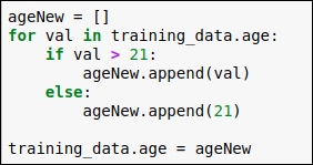
Figure 1.27: Replace the outlier with the minimum age value 21
In the code, you can see that we have checked each data point of the age column, and if the age is greater than 21, then we haven't applied any changes, but if the age is less than 21, then we have replaced the old value with 21. After that, we put all these revised values into our original dataframe.
Number of time 30-59 days past due not worse
In this data attribute, we explore the data as well as referring to the outlier detection graph. Having done that, we know that values 96 and 98 are our outliers. We replace these values with the media value. You can refer to the following code and graph to understand this better.
Refer to the outlier detection graph given in the following figure:
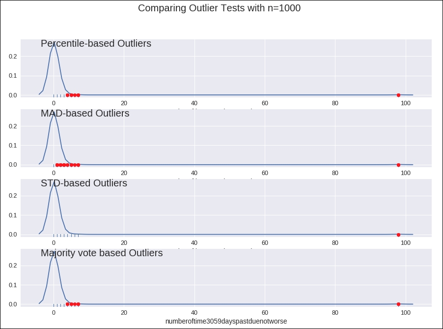
Figure 1.28: Outlier detection graph
Refer to the frequency analysis of the data in the following figure:
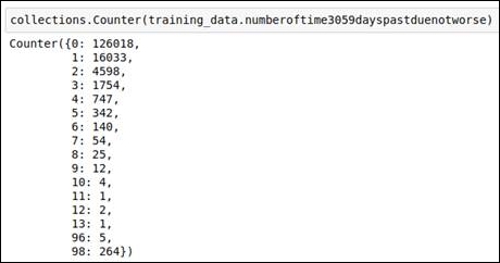
Figure 1.29: Outlier values from the frequency calculation
The code snippet for replacing the outlier values with the median is given in the following figure:

Figure 1.30: Code snippet for replacing outliers
Debt ratio
If we look at the graph of the outlier detection of this attribute, then it's kind of confusing. Refer to the following figure:
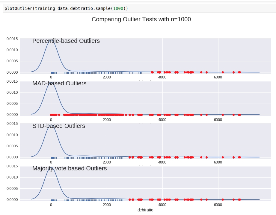
Figure 1.31: Graph of outlier detection for the debt ratio column
Why? It's confusing because we are not sure which outlier detection method we should consider. So, here, we do some comparative analysis just by counting the number of outliers derived from each of the methods. Refer to the following figure:
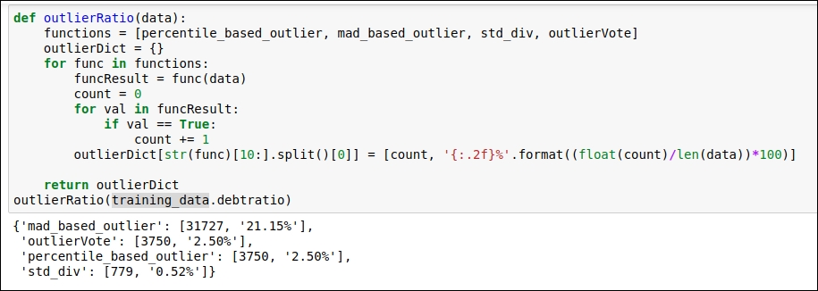
Figure 1.32: Comparison of various outlier detection techniques
The maximum number of outliers was detected by the MAD-based method, so we will consider that method. Here, we will find the minimum upper bound value in order to replace the outlier values. The minimum upper bound is the minimum value derived from the outlier value. Refer to the following code snippet:

Figure 1.33: The code for the minimum upper bound
Monthly income
For this data attribute, we will select the voting-based outlier detection method, as shown in the following figure:
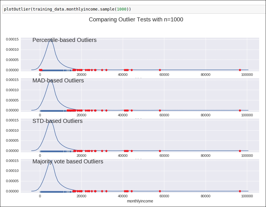
Figure 1.34: Outlier detection graph
In order to replace the outlier, we will use the same logic that we have for the debt ratio data attribute. We replace the outliers by generating a minimum upper bound value. You can refer to the code given in the following figure:
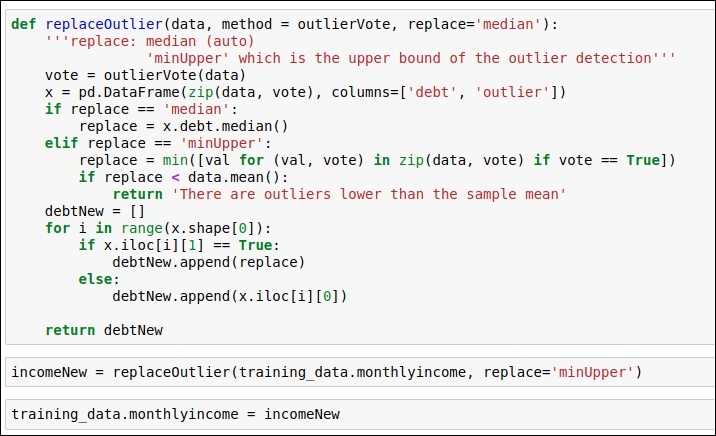
Figure 1.35: Replace the outlier value with the minimum upper bound value
Number of open credit lines and loans
If you refer to the graph given in the following figure, you will see that there are no highly deviated outlier values present in this column:
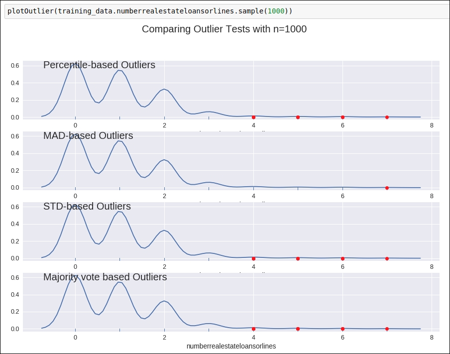
Figure 1.36: Outlier detection graph
So, we will not perform any kind of replacement operation for this data attribute.
Number of times 90 days late
For this attribute, when you analyze the data value frequency, you will immediately see that the values 96 and 98 are outliers. We will replace these values with the median value of the data attribute.
Refer to the frequency analysis code snippet in the following figure:
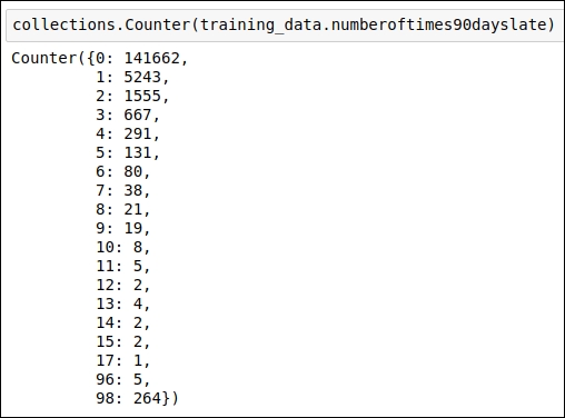
Figure 1.37: Frequency analysis of the data points
The outlier replacement code snippet is shown in the following figure:
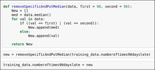
Figure 1.38: Outlier replacement using the median value
Number of real estate loans or lines
When we see the frequency of value present in the data attribute, we will come to know that a frequency value beyond 17 is too less. So, here we replace every value less than 17 with 17.
You can refer to the code snippet in the following figure:

Figure 1.39: Code snippet for replacing outliers
Number of times 60-89 days past due not worse
For this attribute, when you analyze the data value frequency, you will immediately see that the values 96 and 98 are outliers. We will replace these values with the median value of the data attribute.
Refer to the frequency analysis code snippet in the following figure:
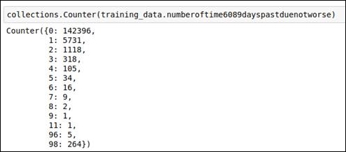
Figure 1.40: Frequency analysis of the data
The outlier replacement code snippet is shown in the following figure:

Figure 1.41: Code snippet for replacing outliers using the median value
You can refer to the removeSpecificAndPutMedian method code from Figure 1.38.
Number of dependents
For this attribute, when you see the frequency value of the data points, you will immediately see that data values greater than 10 are outliers. We replace values greater than 10 with 10.
Refer to the code snippet in the following figure:
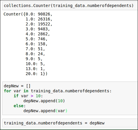
Figure 1.42: Code snippet for replacing outlier values
This is the end of the outlier section. In this section, we've replaced the value of the data points in a more meaningful way. We have also reached the end of our basic data analysis section. This analysis has given us a good understanding of the dataset and its values. The next section is all about feature engineering. So, we will start with the basics first, and later on in this chapter, you will learn how feature engineering will impact the accuracy of the algorithm in a positive manner.


