Search icon CANCEL
Subscription
0
Cart icon
Your Cart (0 item)
Close icon
You have no products in your basket yet
Save more on your purchases! discount-offer-chevron-icon
Savings automatically calculated. No voucher code required.
Arrow left icon
Explore Products
Best Sellers
New Releases
Books
Videos
Audiobooks
Learning Hub
Newsletter Hub
Free Learning
Arrow right icon
timer SALE ENDS IN
0 Days
:
00 Hours
:
00 Minutes
:
00 Seconds
Arrow up icon
GO TO TOP
Jupyter Cookbook

You're reading from   Jupyter Cookbook Over 75 recipes to perform interactive computing across Python, R, Scala, Spark, JavaScript, and more

Arrow left icon
Product type Paperback
Published in Apr 2018
Publisher Packt
ISBN-13 9781788839440
Length 238 pages
Edition 1st Edition
Languages
Tools
Arrow right icon
Author (1):
Arrow left icon
Dan Toomey Dan Toomey
Author Profile Icon Dan Toomey
Dan Toomey
Arrow right icon
View More author details
Toc

Table of Contents (12) Chapters Close

Preface 1. Installation and Setting up the Environment FREE CHAPTER 2. Adding an Engine 3. Accessing and Retrieving Data 4. Visualizing Your Analytics 5. Working with Widgets 6. Jupyter Dashboards 7. Sharing Your Code 8. Multiuser Jupyter 9. Interacting with Big Data 10. Jupyter Security 11. Jupyter Labs

Visualizing with R


There are severalvisualization mechanisms available in R.

  • Produce a R Scatter plot

In this example, we produce a scatter plot using the standard R plot() function. Built into the plot function, we can chart the relationship between the x and y values as well.

How to do it...

We can use this script:

# load the iris dataset
data <- read.csv("http://archive.ics.uci.edu/ml/machine-learning-databases/iris/iris.data")

#Let us also clean up the data so as to be more readable
colnames(data) <- c("sepal_length", "sepal_width", "petal_length", "petal_width", "species")

# make sure the data is as expected
summary(data)
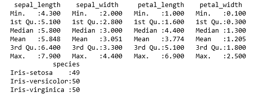
Produce the Scatter plot:

plot(data$sepal_length, data$petal_length)
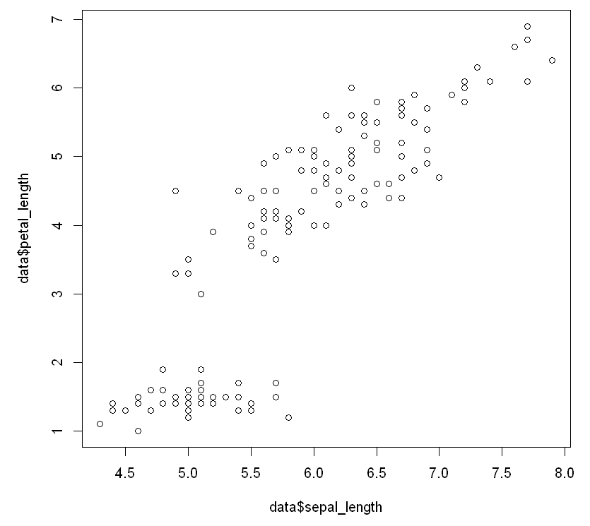
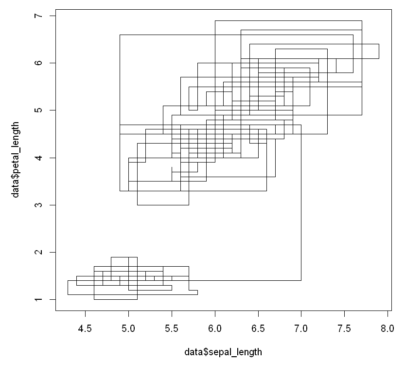
And produce the following visualizations of the relationships between the values. This plot is a stepwise look at how changing one value appears, to see the effect on the other:

plot(data$sepal_length, data$petal_length, type="s")

The output is as follows:
And we look at a histogram of the same data...

lock icon The rest of the chapter is locked
Register for a free Packt account to unlock a world of extra content!
A free Packt account unlocks extra newsletters, articles, discounted offers, and much more. Start advancing your knowledge today.
Unlock this book and the full library FREE for 7 days
Get unlimited access to 7000+ expert-authored eBooks and videos courses covering every tech area you can think of
Renews at $19.99/month. Cancel anytime
Banner background image