Data Quality Assurance and Exploration
So far, we remedied two data quality issues just by asking basic questions or by looking at the .info() summary. Let's now take a look at the first few columns. Before we get to the historical bill payments, we have the credit limits of the accounts of LIMIT_BAL, and the demographic features SEX, EDUCATION, MARRIAGE, and AGE. Our business partner has reached out to us, to let us know that gender should not be used to predict credit-worthiness, as this is unethical by their standards. So we keep this in mind for future reference. Now we explore the rest of these columns, making any corrections that are necessary.
In order to further explore the data, we will use histograms. Histograms are a good way to visualize data that is on a continuous scale, such as currency amounts and ages. A histogram groups similar values into bins, and shows the number of data points in these bins as a bar graph.
To plot histograms, we will start to get familiar with the graphical capabilities of pandas. pandas relies on another library called Matplotlib to create graphics, so we'll also set some options using matplotlib. Using these tools, we'll also learn how to get quick statistical summaries of data in pandas.
Exercise 6: Exploring the Credit Limit and Demographic Features
In this exercise, we start our exploration of data with the credit limit and age features. We will visualize them and get summary statistics to check that the data contained in these features is sensible. Then we will look at the education and marriage categorical features to see if the values there make sense, and correct them as necessary. LIMIT_BAL and AGE are numerical features, meaning they are measured on a continuous scale. Consequently, we'll use histograms to visualize them. Perform the following steps to complete the exercise:
Note
The code and the resulting output for this exercise have been loaded in a Jupyter Notebook that can found here: http://bit.ly/2W9cwPH.
Import matplotlib and set up some plotting options with this code snippet:
import matplotlib.pyplot as plt #import plotting package

#render plotting automatically
%matplotlib inline

import matplotlib as mpl #additional plotting functionality

mpl.rcParams['figure.dpi'] = 400 #high resolution figures
This imports matplotlib and uses .rcParams to set the resolution (dpi = dots per inch) for a nice crisp image; you may not want to worry about this last part unless you are preparing things for presentation, as it could make the images quite large in your notebook.
Run df_clean_2[['LIMIT_BAL', 'AGE']].hist() and you should see the following histograms:
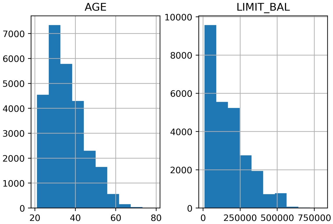
Figure 1.43: Histograms of the credit limit and age data
This is nice visual snapshot of these features. We can get a quick, approximate look at all of the data in this way. In order to see statistics such as mean and median (that is, the 50th percentile), there is another helpful pandas function.
Generate a tabular report of summary statistics using the following command:
df_clean_2[['LIMIT_BAL', 'AGE']].describe()
You should see the following output:
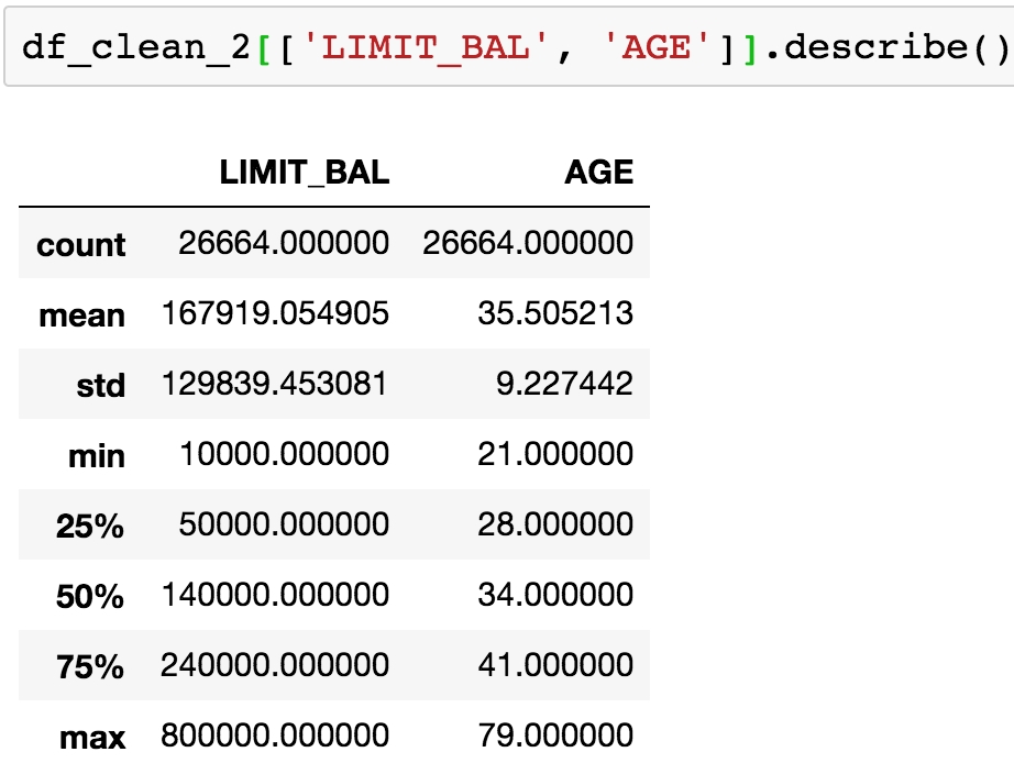
Figure 1.44: Statistical summaries of credit limit and age data
Based on the histograms and the convenient statistics computed by .describe(), which include a count of non-nulls, the mean and standard deviation, minimum, maximum, and quartiles, we can make a few judgements.
LIMIT_BAL, the credit limit, seems to make sense. The credit limits have a minimum of 10,000. This dataset is from Taiwan; the exact unit of currency (NT dollar) may not be familiar, but intuitively, a credit limit should be above zero. You are encouraged to look up the conversion to your local currency and consider these credit limits. For example, 1 US dollar is about 30 NT dollars.
The AGE feature also looks reasonably distributed, with no one under the age of 21 having a credit account.
For the categorical features, a look at the value counts is useful, since there are relatively few unique values.
Obtain the value counts for the EDUCATION feature using the following code:
df_clean_2['EDUCATION'].value_counts()
You should see this output:
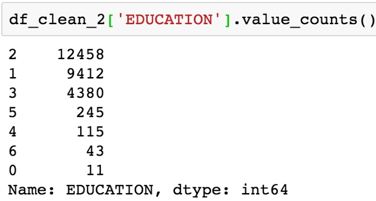
Figure 1.45: Value counts of the EDUCATION feature
Here, we see undocumented education levels 0, 5, and 6, as the data dictionary describes only "Education (1 = graduate school; 2 = university; 3 = high school; 4 = others)". Our business partner tells us they don't know about the others. Since they are not very prevalent, we will lump them in with the "others" category, which seems appropriate, with our client's blessing, of course.
Run this code to combine the undocumented levels of the EDUCATION feature into the level for "others" and then examine the results:
df_clean_2['EDUCATION'].replace(to_replace=[0, 5, 6], value=4, inplace=True)
df_clean_2['EDUCATION'].value_counts()
The pandas .replace method makes doing the replacements described in the preceding step pretty quick. Once you run the code, you should see this output:
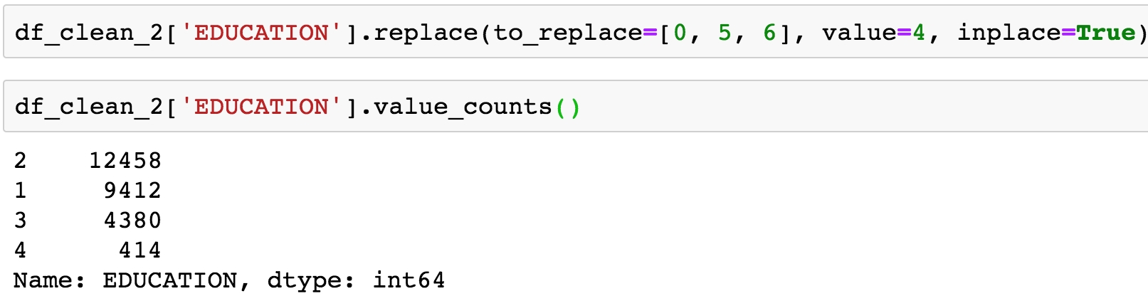
Figure 1.46: Cleaning the EDUCATION feature
Note that here we make this change in place (inplace=True). This means that, instead of returning a new DataFrame, this operation will make the change on the existing DataFrame.
Obtain the value counts for the MARRIAGE feature using the following code:
df_clean_2['MARRIAGE'].value_counts()
You should obtain the following output:
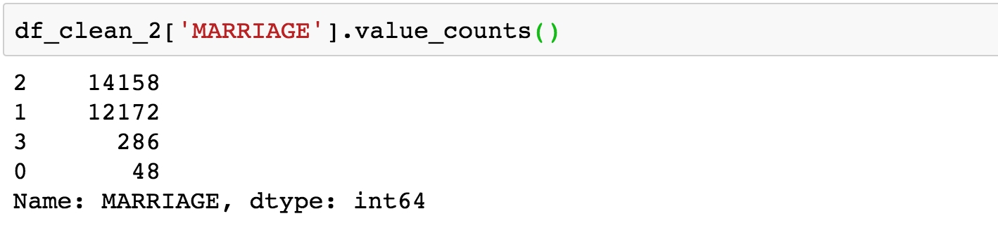
Figure 1.47: Value counts of raw MARRIAGE feature
The issue here is similar to that encountered for the EDUCATION feature; there is a value, 0, which is not documented in the data dictionary: "1 = married; 2 = single; 3 = others". So we'll lump it in with "others".
Change the values of 0 in the MARRIAGE feature to 3 and examine the result with this code:
df_clean_2['MARRIAGE'].replace(to_replace=0, value=3, inplace=True)
df_clean_2['MARRIAGE'].value_counts()
The output should be:
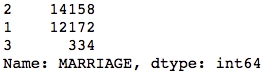
Figure 1.48: Value counts of cleaned MARRIAGE feature
We've now accomplished a lot of exploration and cleaning of the data. We will do some more advanced visualization and exploration of the financial history features, that come after this in the DataFrame, later.
Deep Dive: Categorical Features
Machine learning algorithms only work with numbers. If your data contains text features, for example, these would require transformation to numbers in some way. We learned above that the data for our case study is, in fact, entirely numerical. However, it's worth thinking about how it got to be that way. In particular, consider the EDUCATION feature.
This is an example of what is called a categorical feature: you can imagine that as raw data, this column consisted of the text labels 'graduate school', 'university', 'high school', and 'others'. These are called the levels of the categorical feature; here, there are four levels. It is only through a mapping, which has already been chosen for us, that these data exist as the numbers 1, 2, 3, and 4 in our dataset. This particular assignment of categories to numbers creates what is known as an ordinal feature, since the levels are mapped to numbers in order. As a data scientist, at a minimum you need to be aware of such mappings, if you are not choosing them yourself.
What are the implications of this mapping?
It makes some sense that the education levels are ranked, with 1 corresponding to the highest level of education in our dataset, 2 to the next highest, 3 to the next, and 4 presumably including the lowest levels. However, when you use this encoding as a numerical feature in a machine learning model, it will be treated just like any other numerical feature. For some models, this effect may not be desired.
What if a model seeks to find a straight-line relationship between the features and response?
Whether or not this works in practice depends on the actual relationship between different levels of education and the outcome we are trying to predict.
Here, we examine two hypothetical cases of ordinal categorical variables, each with 10 levels. The levels measure the self-reported satisfaction levels from customers visiting a website. The average number of minutes spent on the website for customers reporting each level is plotted on the y-axis. We've also plotted the line of best fit in each case to illustrate how a linear model would deal with these data, as shown in the following figure:
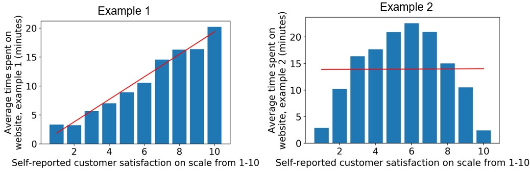
Figure 1.49: Ordinal features may or may not work well in a linear model
We can see that if an algorithm assumes a linear (straight-line) relationship between features and response, this may or may not work well depending on the actual relationship between this feature and the response variable. Notice that in the preceding example, we are modeling a regression problem: the response variable takes on a continuous range of numbers. However, some classification algorithms such as logistic regression also assume a linear effect of the features. We will discuss this in greater detail later when we get into modeling the data for our case study.
Roughly speaking, for a binary classification model, you can look at the different levels of a categorical feature in terms of the average values of the response variable, which represent the "rates" of the positive class (i.e., the samples where the response variable = 1) for each level. This can give you an idea of whether an ordinal encoding will work well with a linear model. Assuming you've imported the same packages in your Jupyter notebook as in the previous sections, you can quickly look at this using a groupby/agg and bar plot in pandas:
f_clean_2.groupby('EDUCATION').agg({'default payment next month':'mean'}).plot.bar(legend=False)
plt.ylabel('Default rate')
plt.xlabel('Education level: ordinal encoding')
Once you run the code, you should obtain the following output:
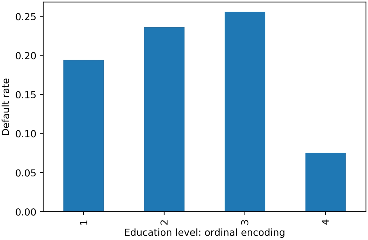
Figure 1.50: Default rate within education levels
Similar to example 2 in Figure 1.49, it looks like a straight-line fit would probably not be the best description of the data here. In case a feature has a non-linear effect like this, it may be better to use a more complex algorithm such as a decision tree or random forest. Or, if a simpler and more interpretable linear model such as logistic regression is desired, we could avoid an ordinal encoding and use a different way of encoding categorical variables. A popular way of doing this is called one-hot encoding (OHE).
OHE is a way to transform a categorical feature, which may consist of text labels in the raw data, into a numerical feature that can be used in mathematical models.
Let's learn about this in an exercise. And if you are wondering why a logistic regression is more interpretable and a random forest is more complex, we will be learning about these concepts in detail during the rest of the book.
Note
Categorical variables in different machine learning packages
Some machine learning packages, for instance, certain R packages or newer versions of the Spark platform for big data, will handle categorical variables without assuming they are ordinal. Always be sure to carefully read the documentation to learn what the model will assume about the features, and how to specify whether a variable is categorical, if that option is available.
Exercise 7: Implementing OHE for a Categorical Feature
In this exercise, we will "reverse engineer" the EDUCATION feature in the dataset to obtain the text labels that represent the different education levels, then show how to use pandas to create an OHE.
First, let's consider our EDUCATION feature, before it was encoded as an ordinal. From the data dictionary, we know that 1 = graduate school, 2 = university, 3 = high school, 4 = others. We would like to recreate a column that has these strings, instead of numbers. Perform the following steps to complete the exercise:
Note
The code and the resulting output for this exercise have been loaded in a Jupyter Notebook that can found here: http://bit.ly/2W9cwPH.
Create an empty column for the categorical labels called EDUCATION_CAT. Using the following command:
df_clean_2['EDUCATION_CAT'] = 'none'
Examine the first few rows of the DataFrame for the EDUCATION and EDUCATION_CAT columns:
df_clean_2[['EDUCATION', 'EDUCATION_CAT']].head(10)
The output should appear as follows:
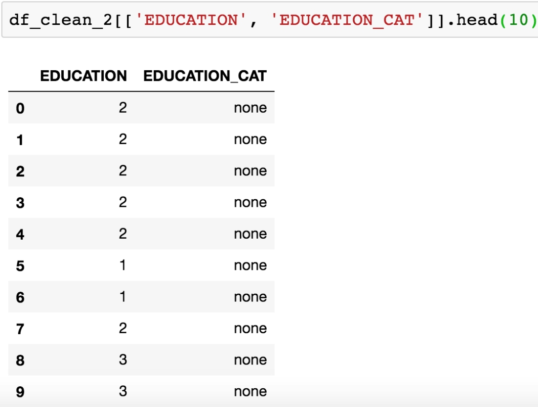
Figure 1.51: Selecting columns and viewing the first 10 rows
We need to populate this new column with the appropriate strings. pandas provides a convenient functionality for mapping values of a Series on to new values. This function is in fact called .map and relies on a dictionary to establish the correspondence between the old values and the new values. Our goal here is to map the numbers in EDUCATION on to the strings they represent. For example, where the EDUCATION column equals the number 1, we'll assign the 'graduate school' string to the EDUCATION_CAT column, and so on for the other education levels.
Create a dictionary that describes the mapping for education categories using the following code:
cat_mapping = {
    1: "graduate school",
    2: "university",
    3: "high school",
    4: "others"
}
Apply the mapping to the original EDUCATION column using .map and assign the result to the new EDUCATION_CAT column:
df_clean_2['EDUCATION_CAT'] = df_clean_2['EDUCATION'].map(cat_mapping)
df_clean_2[['EDUCATION', 'EDUCATION_CAT']].head(10)
After running those lines, you should see the following output:
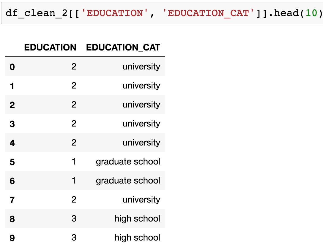
Figure 1.52: Examining the string values corresponding to the ordinal encoding of EDUCATION
Excellent! Note that we could have skipped Step 1, where we assigned the new column with 'none', and gone straight to Steps 3 and 4 to create the new column. However, sometimes it's useful to create a new column initialized with a single value, so it's worth knowing how to do that.
Now we are ready to one-hot encode. We can do this by passing a Series of a DataFrame to the pandas get_dummies() function. The function got this name because one-hot encoded columns are also referred to as dummy variables. The result will be a new DataFrame, with as many columns as there are levels of the categorical variable.
Run this code to create a one-hot encoded DataFrame of the EDUCATION_CAT column. Examine the first 10 rows:
edu_ohe = pd.get_dummies(df_clean_2['EDUCATION_CAT'])
edu_ohe.head(10)
This should produce the following output:
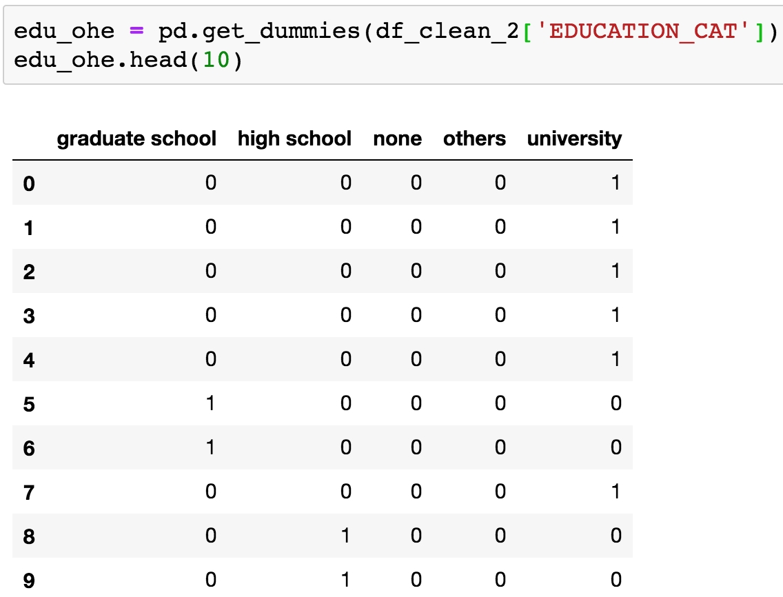
Figure 1.53: Data frame of one-hot encoding
You can now see why this is called "one-hot encoding": across all these columns, any particular row will have a 1 in exactly 1 column, and 0s in the rest. For a given row, the column with the 1 should match up to the level of the original categorical variable. To check this, we need to concatenate this new DataFrame with the original one and examine the results side by side. We will use the pandas concat function, to which we pass the list of DataFrames we wish to concatenate, and the axis=1 keyword saying to concatenate them horizontally; that is, along the column axis. This basically means we are combining these two DataFrames "side by side", which we know we can do because we just created this new DataFrame from the original one: we know it will have the same number of rows, which will be in the same order as the original DataFrame.
Concatenate the one-hot encoded DataFrame to the original DataFrame as follows:
df_with_ohe = pd.concat([df_clean_2, edu_ohe], axis=1)
df_with_ohe[['EDUCATION_CAT', 'graduate school',
             'high school', 'university', 'others']].head(10)
You should see this output:
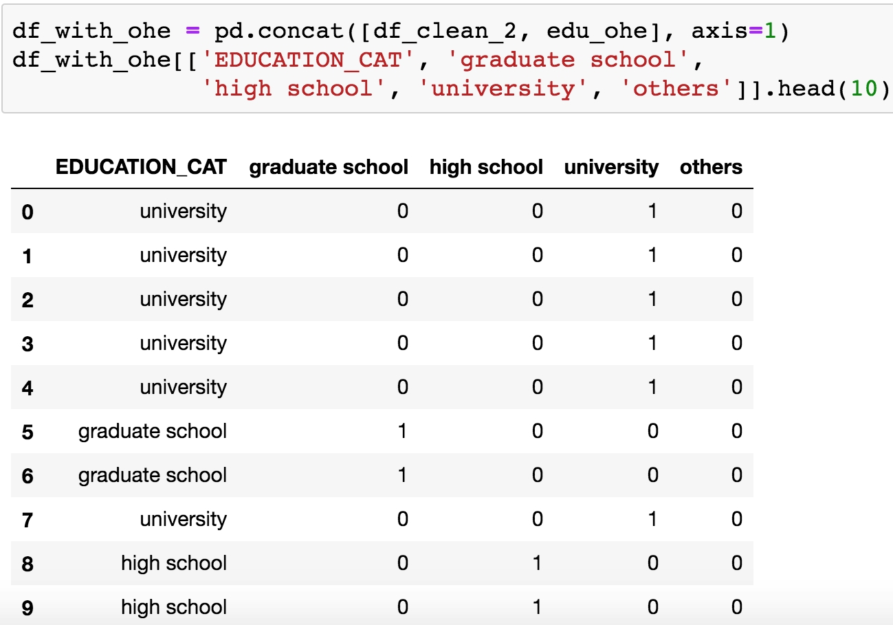
Figure 1.54: Checking the one-hot encoded columns
Alright, looks like this has worked as intended. OHE is another way to encode categorical features that avoids the implied numerical structure of an ordinal encoding. However, notice what has happened here: we have taken a single column, EDUCATION, and exploded it out into as many columns as there were levels in the feature. In this case, since there are only four levels, this is not such a big deal. However, if your categorical variable had a very large number of levels, you may want to consider an alternate strategy, such as grouping some levels together into single categories.
This is a good time to save the DataFrame we've created here, which encapsulates our efforts at cleaning the data and adding an OHE column.
Choose a filename, and write the latest DataFrame to a CSV (comma-separated value) file like this: df_with_ohe.to_csv('../Data/Chapter_1_cleaned_data.csv', index=False), where we don't include the index, as this is not necessary and can create extra columns when we load it later.