Search icon CANCEL
Subscription
0
Cart icon
Your Cart (0 item)
Close icon
You have no products in your basket yet
Save more on your purchases! discount-offer-chevron-icon
Savings automatically calculated. No voucher code required.
Arrow left icon
Explore Products
Best Sellers
New Releases
Books
Videos
Audiobooks
Learning Hub
Newsletter Hub
Free Learning
Arrow right icon
timer SALE ENDS IN
0 Days
:
00 Hours
:
00 Minutes
:
00 Seconds
Arrow up icon
GO TO TOP
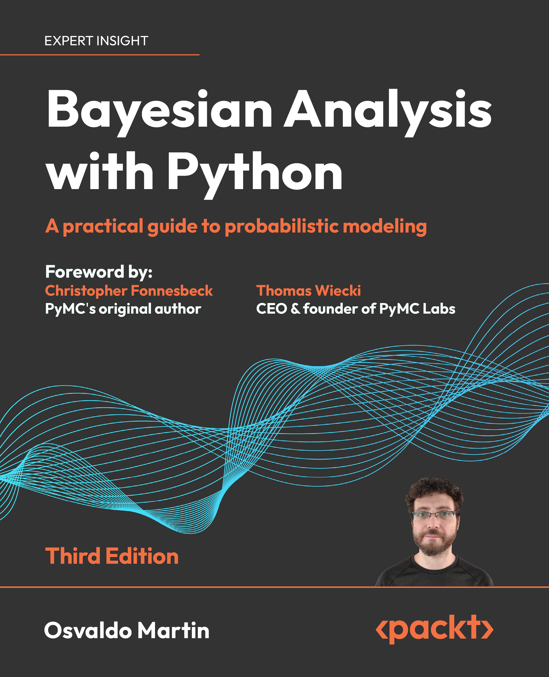
Bayesian Analysis with Python

You're reading from   Bayesian Analysis with Python A practical guide to probabilistic modeling

Arrow left icon
Product type Paperback
Published in Jan 2024
Publisher Packt
ISBN-13 9781805127161
Length 394 pages
Edition 3rd Edition
Languages
Tools
Arrow right icon
Author (1):
Arrow left icon
Osvaldo Martin Osvaldo Martin
Author Profile Icon Osvaldo Martin
Osvaldo Martin
Arrow right icon
View More author details
Toc

Table of Contents (15) Chapters Close

Preface
1. Chapter 1 Thinking Probabilistically FREE CHAPTER 2. Chapter 2 Programming Probabilistically 3. Chapter 3 Hierarchical Models 4. Chapter 4 Modeling with Lines 5. Chapter 5 Comparing Models 6. Chapter 6 Modeling with Bambi 7. Chapter 7 Mixture Models 8. Chapter 8 Gaussian Processes 9. Chapter 9 Bayesian Additive Regression Trees 10. Chapter 10 Inference Engines 11. Chapter 11 Where to Go Next 12. Bibliography
13. Other Books You May Enjoy
14. Index

9.7 Exercises

  1. Explain each of the following:

    • How is BART different from linear regression and splines?

    • When might you want to use linear regression over BART?

    • When might you want to use Gaussian processes over BART?

  2. In your own words, explain why it can be the case that multiple small trees can fit patterns better than one single large tree. What is the difference in the two approaches? What are the trade-offs?

  3. Below, we provide two simple synthetic datasets. Fit a BART model with m=50 to each of them. Plot the data and the mean fitted function. Describe the fit.

    • x = np.linspace(-1, 1., 200) and y = np.random.normal(2*x, 0.25)

    • x = np.linspace(-1, 1., 200) and y = np.random.normal(x**2, 0.25)

    • Create your own synthetic dataset.

  4. Create the following dataset Y = 10sin(πX0X1)+20(X2 0.5)2 +10X3 +5X4 + , where (0,1) and X0:9 (0,1). This is called Friedman’s five-dimensional function. Notice that we actually have 10 dimensions, but the last 5...

lock icon The rest of the chapter is locked
Register for a free Packt account to unlock a world of extra content!
A free Packt account unlocks extra newsletters, articles, discounted offers, and much more. Start advancing your knowledge today.
Unlock this book and the full library FREE for 7 days
Get unlimited access to 7000+ expert-authored eBooks and videos courses covering every tech area you can think of
Renews at $19.99/month. Cancel anytime
Banner background image