Covering the R and RStudio basics
It is easy to confuse R with RStudio if you are a first-time user. In a nutshell, R is the engine that supports all sorts of backend computations, and RStudio is a convenient tool for navigating and managing related coding and reference resources. Specifically, RStudio is an IDE where the user writes R code, performs analysis, and develops models without worrying much about the backend logistics required by the R engine. The interface provided by RStudio makes the development work much more convenient and user-friendly than the vanilla R interface.
First, we need to install R on our computer, as the RStudio will ship with the computation horsepower upon installation. We can choose the corresponding version of R at https://cloud.r-project.org/, depending on the specific type of operating system we use. RStudio can then be downloaded at https://www.rstudio.com/products/rstudio/download/ and installed accordingly. When launching the RStudio application after installing both software, the R engine will be automatically detected and used. Let’s go through an exercise to get familiar with the interface.
Exercise 1.01 – exploring RStudio
RStudio provides a comprehensive environment for working with R scripts and exploring the data simultaneously. In this exercise, we will look at a basic example of how to write a simple script to store a string and perform a simple calculation using RStudio.
Perform the following steps to complete this exercise:
- Launch the RStudio application and observe the three panes:
- The Console pane is used to execute R commands and display the immediate result.
- The Environment pane stores all the global variables in the current session.
- The Files pane lists all the files within the current working directory along with other tabs, as shown in Figure 1.1.
Note that the R version is printed as a message in the console (highlighted in the dashed box):
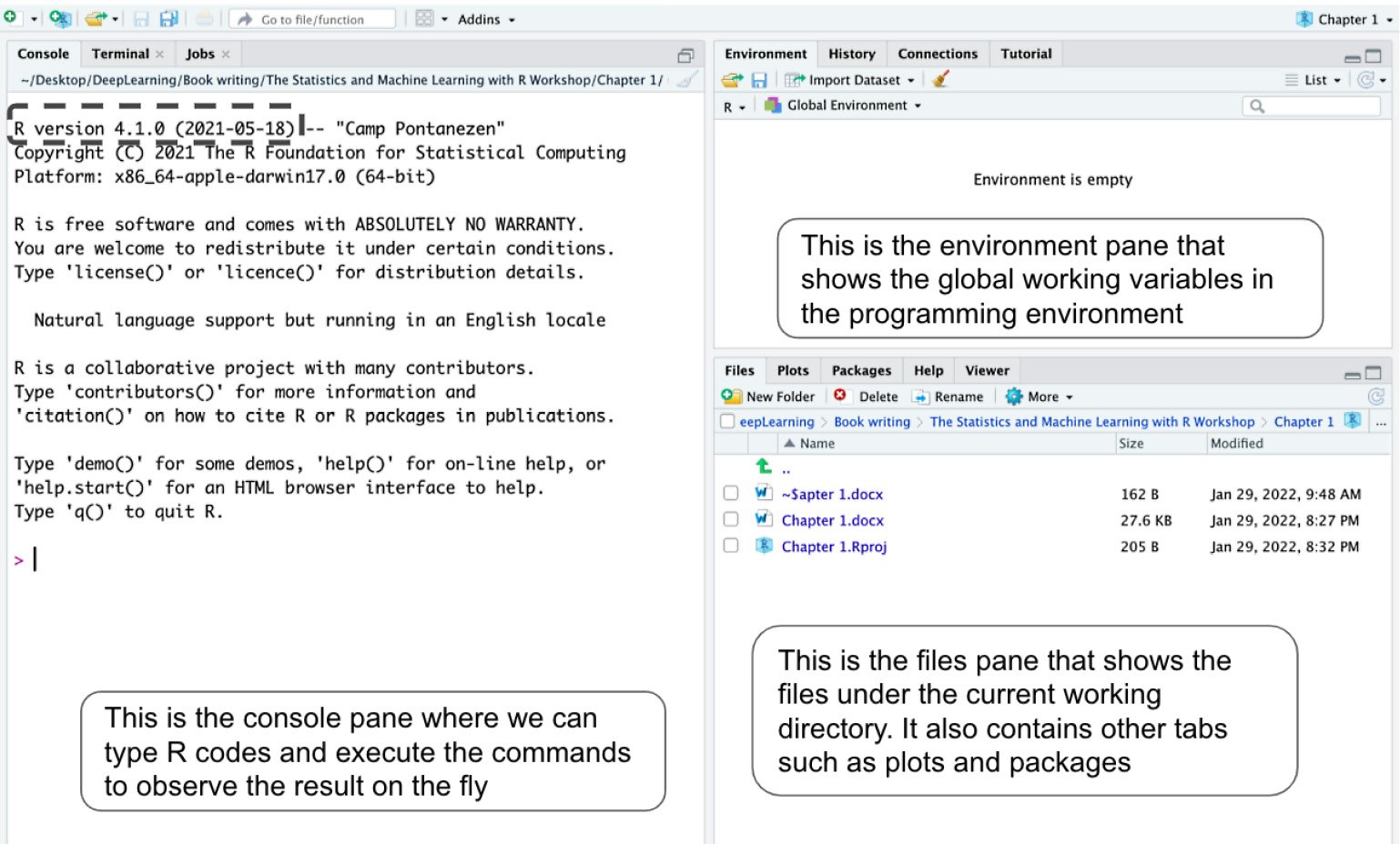
Figure 1.1 – A screenshot of the RStudio upon the first launch
We can also type R.version in the console to retrieve more detailed information on the version of the R engine in use, as shown in Figure 1.2. It is essential to check the R version, as different versions may produce different results when running the same code.
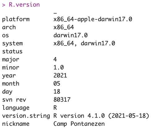
Figure 1.2 – Typing a command in the console to check the R version
- Build a new R script by clicking on the plus sign in the upper-left corner or via File | New File | R Script. An R script allows us to write longer R code that involves functions and chunks of code executed in sequence. We will build an R script and name it
test.Rupon saving the file. See the following figure for an illustration:
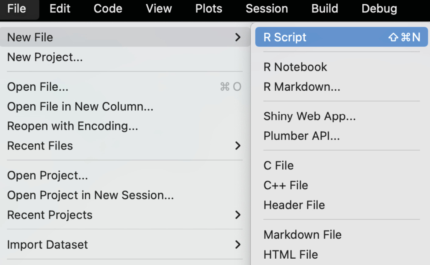
Figure 1.3 – Creating a new R script
- Running the script can be achieved by placing the cursor at the current line and pressing Cmd + Enter for macOS or Ctrl + Enter for Windows; alternatively, click on the Run button at the top of the R script pane, as shown in the following figure:

Figure 1.4 – Executing the script by clicking on the Run button
- Type the following commands in the script editing pane and observe the output in the console as well as the changes in the other panes. First, we create a variable named
testby assigning"I am a string". A variable can be used to store an object, which could take the form of a string, number, data frame, or even function (more on this later). Strings consist of characters, a common data type in R. Thetestvariable created in the script is also reflected in the Environment pane, which is a convenient check as we can also observe the content in the variable. See Figure 1.5 for an illustration:# String assignment test = "I am a string" print(test)

Figure 1.5 – Creating a string-type variable
We also assign a simple addition operation to test2 and print it out in the console. These commands are also annotated via the # sign, where the contents after the sign are not executed and are only used to provide an explanation of the following code. See Figure 1.6 for an illustration:
# Simple calculation
test2 = 1 + 2
print(test2)
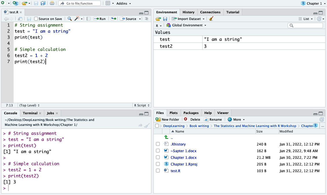
Figure 1.6 – Assigning a string and performing basic computation
- We can also check the contents of the environment workspace via the
ls()function:>>> ls() "test" "test2"
In addition, note that the newly created R script is also reflected in the Files pane. RStudio is an excellent one-stop IDE for working with R and will be the programming interface for this book. We will introduce more features of RStudio in a more specific context along the way.
Note
The canonical way of assigning some value to a variable is via the <- operator instead of the = sign as in the example. However, the author chose to use the = sign as it is faster to type on the screen and has an equivalent effect as the <- sign in the majority of cases.
In addition, note that the output message in the Console pane has a preceding [1] sign, which indicates that the result is a one-dimensional output. We will ignore this sign in the output message unless otherwise specified.
The exercise in the previous section provides an additional example, which is an essential operation in R. As with other modern programming languages, R also ships with many standard arithmetic operators, including subtraction (-), multiplication (*), division (/), exponentiation (^), and modulo (%%) operators. The modulo operator returns the remainder of the numerator in the division operation.
Let’s look at an exercise to go through some common arithmetic operations.
Exercise 1.02 – common arithmetic operations in R
This exercise will perform different arithmetic operations (addition, subtraction, multiplication, division, exponentiation, and modulo) between two numbers: 5 and 2.
Type the commands under the EXERCISE 1.02 comment section in the R Script pane and observe the output message in the console shown in Figure 1.7. Note that we removed the print() function, as directly executing the command will also print out the result as highlighted in the console:
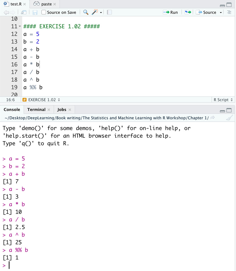
Figure 1.7 – Performing common arithmetic operations in R
Note that these elementary arithmetic operations can jointly form complex operations. When evaluating a complex operation that consists of multiple operators, the general rule of thumb is to use parentheses to enforce the execution of a specific component according to the desired sequence. This follows in most numeric analyses using any programming language.
But, what forms can we expect the data to take in R?
Common data types in R
There are five most basic data types in R: numeric, integer, character, logical, and factor. Any complex R object can be decomposed into individual elements that fall into one of these five data types and, therefore, contain one or more data types. The definition of these five data types is as follows:
- Numeric is the default data type in R and represents a decimal value, such as
1.23. A variable is treated as a numeric even if we assign an integer value to it in the first place. - Integer is a whole number and so a subset of the numeric data type.
- Character is the data type used to store a sequence of characters (including letters, symbols, or even numbers) to form a string or a piece of text, surrounded by double or single quotes.
- Logical is a Boolean data type that only takes one of two values:
TRUEorFALSE. It is often used in a conditional statement to determine whether specific codes after the condition should be executed. - Factor is a special data type used to store categorical variables that contain a limited number of categories (or levels), ordered or unordered. For example, a list of student heights classified as low, medium, and high can be represented as a factor type to encode the inherent ordering, which would not be available when represented as a character type. On the other hand, unordered lists such as male and female can also be represented as factor types.
Let’s go through an example to understand these different data types.
Exercise 1.03 – understanding data types in R
R has strict rules on the data types when performing arithmetic operations. In general, the data types of all variables should be the same when evaluating a particular statement (a piece of code). Performing an arithmetic operation on different data types may give an error. In this exercise, we will look at how to check the data type to ensure the type consistency and different ways to convert the data type from one into another:
- We start by creating five variables, each belonging to a different data type. Check the data type using the
class()function. Note that we can use the semicolon to separate different actions:>>> a = 1.0; b = 1; c = "test"; d = TRUE; e = factor("test") >>> class(a); class(b); class(c); class(d); class(e) "numeric" "numeric" "character" "logical" "factor"As expected, the data type of the
bvariable is converted into numeric even when it is assigned an integer in the first place. - Perform addition on the variables. Let’s start with the
aandbvariables:>>> a + b 2 >>> class(a + b) "numeric"
Note that the decimal point is ignored when displaying the result of the addition, which is still numeric as verified via the
class()function.Now, let’s look at the addition between
aandc:>>> a + c Error in a + c : non-numeric argument to binary operator
This time, we received an error message due to a mismatch in data types when evaluating an addition operation. This is because the
+addition operator in R is a binary operator designed to take in two values (operands) and produce another, all of which need to be numeric (including integer, of course). The error pops up when any of the two input arguments are non-numeric. - Let’s trying adding
aandd:>>> a + d 2 >>> class(a + d) "numeric"
Surprisingly, the result is the same as
a + b, suggesting that the Booleanbvariable taking aTRUEvalue is converted into a value of one under the hood. Correspondingly, a Boolean value ofFALSE, obtained by adding an exclamation mark before the variable, would be treated as zero when performing an arithmetic operation with a numeric:>>> a + !d 1
Note that the implicit Boolean conversion occurs in settings when such conversion is necessary to proceed in a specific statement. For example,
dis converted into a numeric value of one when evaluating whetheraequalsd:>>> a == d TRUE
- Convert the data types using the
as.(datatype)family of functions in R.For example, the
as.numeric()function converts the input parameter into a numeric,as.integer()returns the integer part of the input decimal,as.character()converts all inputs (including numeric and Boolean) into strings, andas.logical()converts any non-zero numeric intoTRUEand zero intoFALSE. Let’s look at a few examples:>>> class(as.numeric(b)) "numeric"
This suggests that the
bvariable is successfully converted into numeric. Note that type conversion is a standard data processing operation in R, and type incompatibility is a popular source of error that may be difficult to trace:>>> as.integer(1.8) 1 >>> round(1.8) 2
Since
as.integer()only returns the integer part of the input, the result is always “floored” to the lower bound integer. We could use theround()function to round it up or down, depending on the value of the first digit after the decimal point:>>> as.character(a) "1" >>> as.character(d) "TRUE"
The
as.character()function converts all input parameters into strings as represented by the double quotes, including numeric and Boolean. The converted value no longer maintains the original arithmetic property. For example, a numeric converted into a character would not go through the addition operation. Also, a Boolean converted into a character would no longer be evaluated via a logical statement and treated as a character:>>> as.factor(a) 1 Levels: 1 >>> as.factor(c) test Levels: test
Since there is only one element in the input parameter, the resulting number of levels is only
1, meaning the original input itself.
Note
A categorical variable is called a nominal variable when there is no natural ordering among the categories, and an ordinal variable if there is natural ordering. For example, the temperature variable valued as either high, medium, or low has an inherent ordering in nature, while a gender variable valued as either male or female has no order.


