


1.3 Pure and Mixed States
There are situations where the state of a quantum mechanical system cannot be described with the help of a state vector. Here, we look at such situations and provide a mathematical tool for describing them.
1.3.1 Density matrix
Let us start with the state of a combined two-component physical system given by (1.2.5). Let ( )i=1,...,N and (
 )j=1,...,M denote, respectively, the standard orthonormal bases of the Hilbert spaces of systems A and B:
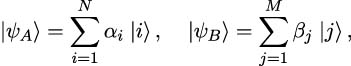
|
where (αi)i=1,...,N and (βj)j=1,...,M are some probability amplitudes. The states that allow the state vector representation (1.3.1) are called pure states. In this case, the state of the combined system is
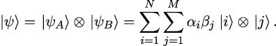
|
However, in general, the state of the combined system would look like
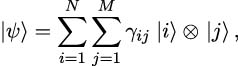
|
where γij are probability amplitudes that may not necessarily be factorised as the product of probability amplitudes (αi)i=1,...,N and (βj)j=1,...,M. If γij cannot be factorised as αiβj, then the component systems A and B are entangled and their states cannot be represented by the state vectors (1.3.1). Such states of systems A and B are called mixed states.
The more general setup is that of an ensemble of states of the form {pk, }k=1,…,N, where each
  is a quantum state whose wavefunction is known with certainty (although this does not necessarily provide full knowledge of the measurement statistics), and each pk is the associated probability (not amplitude) in [0,1]. In order to define properly pure and mixed states, introduce the density operator as follows:
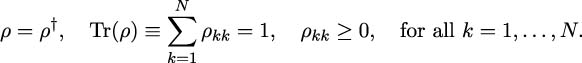
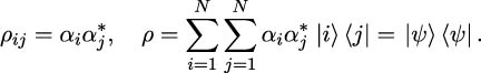
Definition 7. A density operator ρ is a positive semidefinite Hermitian operator with unit trace and takes the form
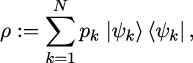
|
where ∑ k=1Npk = 1 and  equals 1 if k = l and zero otherwise.
Mathematically, such a density operator ρ corresponds to a density matrix (ρkl)k,l=1,…,N such that
1.3.2 Pure state
A pure state is one that can be represented by a state vector
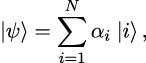
|
where (αi)i=1,...,N are probability amplitudes in ℂ such that ∑ i=1N|αi|2 = 1. In the ensemble setup above, this means that there exists k∗∈{1,…,N} such that pk∗ = 1 and hence  =
=  and therefore ρ =
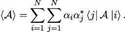
  ⟨ψ|. The density matrix also allows us to compute expectations of the form (1.2.4):
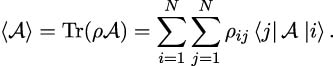
Lemma 3. Let ρ be the density matrix associated to the pure state (1.3.2) and let 𝒜 be an observable (Hermitian operator), then

Proof. The lemma follows from the immediate computation
⟨ψ|𝒜 |
= ⟨ψ|𝒜∑ i=1Nα i |
= ∑ i=1Nα i ⟨ψ|𝒜 |
|
= ∑ i=1N ⟨ψ|𝒜 ⟨ψ|𝒜 |
|
= ∑ i=1N ⟨i|ρ𝒜 = Tr(ρ𝒜). = Tr(ρ𝒜). |
With the state  given by (1.3.2), we obtain
|
At the same time we have
|
Comparison of (1.3.2) and (1.3.2) yields the following expression for the density matrix of a pure state:
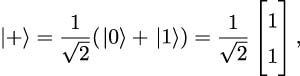
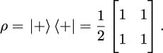
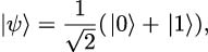
Example: An example of a pure state is the Hadamard state
with corresponding density matrix
1.3.3 Mixed state
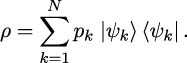
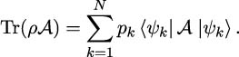
A mixed state is one that cannot be represented by a single pure state vector, and is therefore represented as a statistical distribution of pure states in the form of an ensemble of quantum states {pk, }k=1,…,N, where ∑ k=1Npk = 1 and pk ∈ [0,1] for each k. The density of a mixed state therefore reads
|
Similarly to Lemma 3, we can write expectations of observables with respect to mixed states using the density matrix:
Lemma 4. Let ρ be the density matrix associated to the mixed state (1.3.3) and let 𝒜 be an observable (Hermitian operator), then
Proof. The lemma follows from the immediate computation
| Tr(ρ𝒜) | = ∑ i=1N ⟨i|ρ𝒜 |
= ∑ i=1N ⟨i|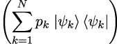 𝒜 𝒜 |
|
= ∑ k=1Np k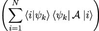 |
|
= ∑ k=1Np k ⟨ψk|𝒜 . . |
Let us see now how the density matrix formalism can help us describe the state of a combined system. Consider an entangled state of two systems, A and B, given by (1.3.1), and a Hermitian operator 𝒜 that only acts within the Hilbert space of system A. What would be the expectation value of 𝒜 in this state? Starting with (1.2.4), we obtain
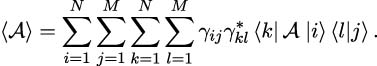
|
Since only terms with l = j survive in (1.3.3) due to the orthogonality of the basis states, we have
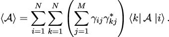
|
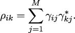
Thus, the density matrix that describes the mixed state of system A is
Note that in the case where the probability amplitudes γij can be factorised as the product of probability amplitudes (αi)i=1,...,N and (βj)j=1,...,M, we obtain
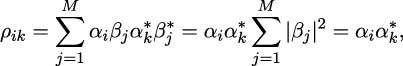
which describes a pure state.
A simple criterion to distinguish a pure state from a mixed state is the following:
Lemma 5. Let ρ be a density matrix. The inequality Tr(ρ2) ≤ 1 always holds and Tr(ρ2) = 1 if and only if ρ corresponds to a pure state.
Proof. Consider an ensemble of pure states {pi, }i=1,…,N, with density matrix given by (1.3.3). Therefore
| Tr(ρ2) | = Tr |
= Tr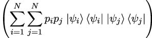 |
|
= Tr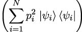 = ∑ i=1Np i2Tr = ∑ i=1Np i2Tr  ⟨ψi| ⟨ψi| = ∑ i=1Np i2 = ∑ i=1Np i2 = ∑ i=1Np i2, = ∑ i=1Np i2, |
which is smaller than 1 since the pi are probabilities in [0,1] summing up to 1. Assume now that Tr(ρ2) equals one, then so does ∑ i=1Npi2. If pi ∈ (0,1) for all i = 1,…,N, then
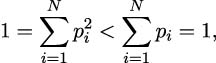
which is a contradiction, and therefore there exists i∗∈{1,…,N} such that pi∗ = 1, so that ρ =  ⟨ψi∗| is a pure state. Conversely, if ρ =
  ⟨ψi| for some i ∈{1,…,N} represents a pure state, then

Example: An example of a mixed state is a statistical ensemble of states  and
and  . If a physical system is prepared to be either in state
  or state
  with equal probability, it can be described by the mixed state
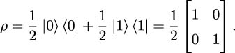
|
Note that this is different from the density matrix of the pure state
which reads

Unlike pure quantum states, mixed quantum states cannot be described by a single state vector. However, the pure states and the mixed states can be described by the density matrix.


