Depth-first search (DFS)

In short, graph searches traverse a graph to map its structure. In this section, we will learn about an algorithm to accomplish such a search. Mapping out the structure of a graph can be important on its own, but it is a sub-problem that algorithms must solve in order to solve larger problems in graphs, as we have discussed. The DFS algorithm is quite possibly the most common approach for graph searches; it is an efficient method, and it is used as a subroutine in many more complex algorithms.

DFS starts at a source vertex, traverses the first available edge to visit another vertex, and repeats this until there are no edges leading to unvisited vertices—that is, until it has gone as deep as possible. At this time, it backtracks to the last vertex that has unvisited neighbors and takes another trip from that vertex through as many unvisited vertices until it reaches another dead end. It then backtracks and travels to unvisited vertices again and again until all the vertices connected to the source have been visited.

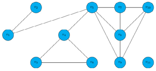
Let's pursue this method on the following small graph so that we can understand the idea well. We will start at v1 and explore the graph using DFS.

Note that it was not specified how to choose a path, so we will arbitrarily move to the lowest-numbered vertex when we have more than one option. We will color vertices and edges within the current path orange and previously visited vertices and previously traversed edges will be green:

Figure 9.1 – A graph

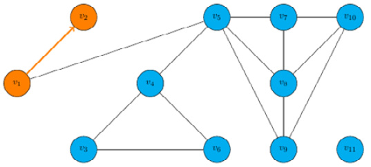
Step 1: The first step will go to v2, which is not adjacent to any vertices we have not yet visited, so it stops:

Figure 9.2 – Step 1 of DFS

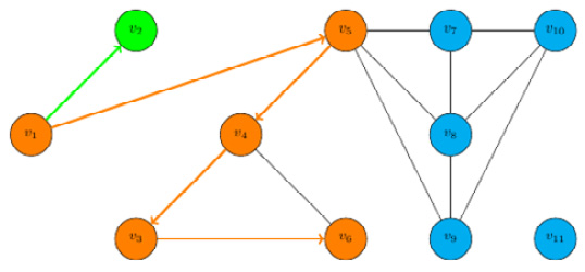
Step 2: We backtrack to node v1, and then follow paths until we reach a dead end once again. This will take us from v1 to v5 to v4 to v3 to v6, which has no unvisited neighbors, so we stop:

Figure 9.3 – Step 2 of DFS

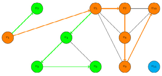
Step 3: We backtrack all the way to v5 because it is the latest one in the orange path with unvisited neighbors and take a path to v7 to v8 to v9 to v10 and stop:

Figure 9.4 – Step 3 of DFS

Finally, all the vertices connected to source v1 are colored in our diagram, indicating all have been visited, so the graph search is complete.

The list of vertices this DFS would produce is as follows:

Notice vertex v11 has not been visited because it is not connected to the source vertex. In general, DFS will not leave a connected component of the source vertex. For a graph with multiple connected components, you would have to run DFS once within each component if you wanted to visit all the vertices.

Now, let's move on to write an implementation of the DFS algorithm in Python.

A Python implementation of DFS

Of course, for large, practical problems, we cannot simply apply the algorithm by hand! Instead, let's write an implementation of the DFS algorithm in Python.

We will write a function called DFS that will take an input of an adjacency matrix of a graph and will return all the vertices connected by a path to the source vertex.

We will present it in pieces and explain as we go. First, we have some documentation listing what the function does and outlines its inputs and outputs:

# Depth First Search
# 
# INPUTS
# A - an adjacency matrix. It should be square, symmetric, and 
  # binary
# source - the number of the source vertex
#
# OUTPUTS
# vertexList - an ordered list of vertices found in the search

Next, we define the functions with inputs of an adjacency matrix and source vertex, subtract the source by 1 since Python counts from 0, find the number of vertices in the graph, and initialize several data structures, including a binary array to store which vertices have been visited, a stack to be used in the algorithm, and a vertex list the algorithm will fill in:

def DFS(A, source):
    # reduce the source by 1 to avoid off-by-1 errors
    source -= 1
    
    # find the number of vertices
    n = A.shape[0]
    
    # initialize the unvisited vertex set to be full
    unvisited = [1] * n
    
    # initialize a queue with the source vertex
    stack = [source]
    
    # initialize the vertex list
    vertexList = []

Then, take the last vertex in the stack and add it to the vertex list if it has not been visited, and add all unvisited neighboring vertices to the end of the queue. Repeat this until the stack is empty. And, lastly, return the vertex list:

    # while the stack is not empty
    while stack:
        # remove the just-visited vertex from the stack and 
          # store it
        v = stack.pop()
        
        # if v is unvisited, add it to our list and mark it as 
          # visited
        if unvisited[v]:
            # save and print the number of the newly visited 
               # vertex
            vertexList.append(v)
            
            # mark the vertex as visited
            unvisited[v] = 0
        # iterate through the vertices
        for u in range(n - 1, 0, -1):
            # add each unvisited neighbor to the stack
            if A[v,u] == 1 and unvisited[u] == 1:
                stack.append(u)
                
    return vertexList

Now that the code is written, let's test it on the example we did previously by hand just to confirm it works as intended. We will need to save the adjacency matrix first:

# Save the adjacency matrix for the graph in Figure 9.1
A = numpy.array([[0, 1, 0, 0, 1, 0, 0, 0, 0, 0, 0],
                  [1, 0, 0, 0, 0, 0, 0, 0, 0, 0, 0],
                  [0, 0, 0, 1, 0, 1, 0, 0, 0, 0, 0],
                  [0, 0, 1, 0, 1, 1, 0, 0, 0, 0, 0],
                  [1, 0, 0, 1, 0, 0, 1, 1, 1, 0, 0],
                  [0, 0, 1, 1, 0, 0, 0, 0, 0, 0, 0],
                  [0, 0, 0, 0, 1, 0, 0, 1, 0, 1, 0],
                  [0, 0, 0, 0, 1, 0, 1, 0, 1, 1, 0],
                  [0, 0, 0, 0, 1, 0, 0, 1, 0, 1, 0],
                  [0, 0, 0, 0, 0, 0, 1, 1, 1, 0, 0],
                  [0, 0, 0, 0, 0, 0, 0, 0, 0, 0, 0]])

Next, let's run the DFS algorithm with source vertex 1 just like we did by hand before. We will also add 1 to each of the numbers in the vertex list since we have counted from 1 unlike Python:

# Run DFS on the graph with adjacency matrix A and source 1
vertexList = DFS(A,1)
# Add 1 to the vertex numbers
[x + 1 for x in vertexList]

The output is as follows:

[1, 2, 5, 4, 3, 6, 7, 8, 9, 10]

When we applied the algorithm by hand, note that we found the exact same list in the exact same order. Clearly, the code is replicating what we were able to do by hand except it runs almost instantly, so our DFS implementation is a great success!

In this section, we have learned what the DFS algorithm is, discussed some of its applications, applied it by hand to an example, wrote a Python implementation of the algorithm, and showed that it matches the results of our example.

The remainder of the chapter focuses on a very practical problem: finding the shortest path between two vertices in a network or weighted graph.