ML development life cycle

The ML development life cycle is a process to create and take to production an application containing an ML model that solves a business problem. The ML model can then be served to customers through the application as part of a product or service offering.

The following diagram illustrates the ML development life cycle process:

Defining problem and objectives

Before any development begins, the problem to be solved must be defined together with objectives of what good will look like, to set expectations. The way the problem is formulated is very important, as this can mean the difference between intractability and a simple solution. It is also likely to involve a conversation about where the input data for any algorithm will come from.

ML algorithms usually require large amounts of data to perform at their best. Sourcing quality data is the most important consideration when planning a ML project.

The typical formulation of an ML problem takes the form given X dataset, predict Y. The availability of data or lack of it thereof can affect the formulation of the problem, the solution, and its feasibility. For example, consider the problem given a large labeled set of images of handwritten digits^[18], predict the label of a previously unseen image. Deep learning algorithms have demonstrated that it is possible to achieve relatively high accuracy on this particular problem with little work on the part of the engineer, as long as the training dataset is sufficiently large^[19]. If the training set is not large, the problem immediately becomes more difficult and requires a careful selection of the algorithm to use. It also affects the accuracy and thus, the set of attainable objectives.

Experiments performed by Michael Nielsen on the MNIST handwritten digit dataset show that the difference between training an ML algorithm with 1 example of labeled input/output pairs per digit and 5 examples was an improvement of accuracy from around 40% to around 65% for most algorithms tested^[20]. Using 10 examples per digit usually raised the accuracy a further 5%.

If insufficient data is available to meet the project objectives, it is sometimes possible to boost performance by artificially expanding the dataset by making small changes to existing examples. In the previously mentioned experiments, Nielsen observed that adding slightly rotated or translated images to the dataset improved performance by as much as 15%.

Acquiring and exploring data

We argued earlier that it is critical to understand the input dataset before specifying project objectives, particularly objectives related to accuracy. As a general rule, ML algorithms will produce the best results when there are large training datasets available. The more data is used to train them, the better they will perform.

Acquiring data is, therefore, a key step in the ML development life cycle—one that can be very time-consuming and fraught with difficulty. In certain industries, privacy legislation may cause a lack of availability of personal data, making it difficult to create personalized products or requiring anonymization of source data before it can be used. Some datasets may be available but could require such extensive preparation or even manual labeling that it may put the project timeline or budget under stress.

Even if you do not have a proprietary dataset to apply to your problem, you may be able to find public datasets to use. Often, public datasets will have received attention from researchers, so you may find that the particular problem you are attempting to tackle has already been solved and the solution is open source. Some good sources of public datasets areas follows:

• Awesome datasets: https://github.com/awesomedata/awesome-public-datasets
• Skymind open datasets: https://skymind.ai/wiki/open-datasets
• OpenML: https://www.openml.org/
• Kaggle: https://www.kaggle.com/datasets
• UK Governments open data: https://data.gov.uk/
• US Governments open data: https://www.data.gov/

Once the dataset has been acquired, it should be explored to gain a basic understanding of how the different features (independent variables) may affect the desired output. For example, when attempting to predict correct height and weight from self-reported figures, researchers determined from initial exploration that older subjects were more likely to under-report obesity and therefore that age was thus a relevant feature when building their model. Attempting to build a model from all available data, even features that may not be relevant, can lead to longer training times in the best case, and can severely hamper accuracy in the worst case by introducing noise.

It is worth spending a bit more time to process and transform a dataset as this will improve the accuracy of the end result and maybe even the training time. All the code examples in this book include data processing and transformation.

In Chapter 2, Setting Up the ML Environment, we will see how to explore data using Go and an interactive browser-based tool called Jupyter.

Selecting the algorithm

The selection of the algorithm is arguably the most important decision that an ML application engineer will need to make, and the one that will take the most research. Sometimes, it is even required to combine an ML algorithm with traditional computer science algorithms to make a problem more tractable—an example of this is a recommender system that we consider later.

A good first step to start homing in on the best algorithm to solve a given problem is to determine whether a supervised or unsupervised approach is required. We introduced both earlier in the chapter. As a rule of thumb, when you are in possession of a labeled dataset and wish to categorize or predict a previously unseen sample, this will use a supervised algorithm. When you wish to understand an unlabeled dataset better by clustering it into different groups, possibly to then classify new samples against, you will use an unsupervised learning algorithm. A deeper understanding of the advantages and pitfalls of each algorithm and a thorough exploration of your data will provide enough information to select an algorithm. To help you get started, we cover a range of supervised learning algorithms in Chapter 3, Supervised Learning, and unsupervised learning algorithms in Chapter 4, Unsupervised Learning.

Some problems can lend themselves to a deft application of both ML techniques and traditional computer science. One such problem is recommender systems, which are now widespread in online retailers such as Amazon and Netflix. This problem asks, given a dataset of each users set of purchased items, predict a set of N items that the user is most likely to purchase next. This is exemplified in Amazons people who buy X also buy Y system.

The basic idea of the solution is that, if two users purchase very similar items, then any items not in the intersection of their purchased items are good candidates for their future purchases. First, transform the dataset so that it maps pairs of items to a score that expresses their co-occurrence. This can be computed by taking the number of times that the same customer has purchased both items, divided by the number of times a customer has purchased either one or the other, to give a number between 0 and 1. This now provides a labeled dataset to train a supervised algorithm such as a binary classifier to predict the score for a previously unseen pair. Combining this with a sorting algorithm can produce, given a single item, a list of items in a sorted rank of purchasability.

Preparing data

Data preparation refers to the processes performed on the input dataset before training the algorithm. A rigorous preparation process can simultaneously enhance the quality of the data and reduce the amount of time it will take the algorithm to reach the desired accuracy. The two steps to preparing data are data pre-processing and data transformation. We will go into more detail on preparing data in Chapters 2, Setting Up The Development Environment, Chapter 3, Supervised Learning, and Chapter 4, Unsupervised Learning.

Data pre-processing aims to transform the input dataset into a format that is adequate for work with the selected algorithm. A typical example of a pre-processing task is to format a date column in a certain way, or to ingest CSV files into a database, discarding any rows that lead to parsing errors. There may also be missing data values in an input data file that need to either be filled in (say, with a mean), or the entire sample discarded. Sensitive information such as personal information may need to be removed.

Data transformation is the process of sampling, reducing, enhancing, or aggregating the dataset to make it more suitable for the algorithm. If the input dataset is small, it may be necessary to enhance it by artificially creating more examples, such as rotating images in an image recognition dataset. If the input dataset has features that the exploration has deemed irrelevant, it would be wise to remove them. If the dataset is more granular than the problem requires, aggregating it to a coarser granularity may help speed up results, such as aggregating city-level data to counties if the problem only requires a prediction per county.

Finally, if the input dataset is particularly large, as is the case with many image datasets intended for use by deep learning algorithms, it would be a good idea to start with a smaller sample that will produce fast results so that the viability of the algorithm can be verified before investing in more computing resources.

The sampling process will also divide the input dataset into training and validation subsets. We will explain why this is necessary later, and what proportion of the data to use for both.

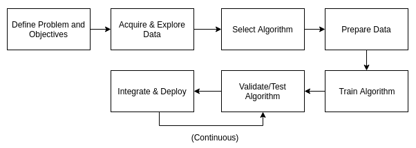
Training

The most compute-intensive part of the ML development life cycle is the training process. Training an ML algorithm can take seconds in the simplest case or days when the input dataset is enormous and the algorithm requires many iterations to converge. The latter case is usually observed with deep learning techniques. For example, DeepMinds AlphaGo Zero algorithm took forty days to fully master the game of Go, even though it was proficient after only three^[22]. Many algorithms that operate on smaller datasets and problems other than image or sound recognition will not require such a large amount of time or computational resource.

Cloud-based computational resources are getting cheaper and cheaper, so, if an algorithm, especially a deep learning algorithm, is taking too long to train on your PC, you can deploy and train it on a cloud instance for a few dollars. We will cover deployment models in Chapter 6, Deploying Machine Learning Applications.

While the algorithm is training, particularly if the training phase will take a long time, it is useful to have some real-time measures of how well the training is going, so that it can be interrupted, re-configured, and restarted without waiting for the training to complete. These metrics are typically classified as loss metrics, where loss refers to the notional error that the algorithm makes either on the training or validation subsets.

Some of the most common loss metrics in prediction problems are as follows:

• Mean square error (MSE) measures the sum of the squared distance between the output variable and the predicted values.
• Mean absolute error (MAE) measures the sum of the absolute distance between the output variable and the predicted values.
• Huber loss is a combination of the MSE and MAE that is more robust to outliers while remaining a good estimator of both the mean and median loss.

Some of the most common loss metrics in classification problems are as follows:

• Logarithmic loss measures the accuracy of the classifier by placing a penalty on false classifications. It is closely related to cross-entropy loss.
• Focal loss is a newer loss func aimed at preventing false negatives when the input dataset is sparse^[23].

Validating/testing

Software engineers are familiar with testing and debugging software source code, but how should ML models be tested? Pieces of algorithms and data input/output routines can be unit tested, but often it is unclear how to ensure that the ML model itself, which presents as a black box, is correct.

The first step to ensuring correctness and sufficient accuracy of an ML model is validation. This means applying the model to predict or classify the validation data subset, and measuring the resulting accuracy against project objectives. Because the training data subset was already seen by the algorithm, it cannot be used to validate correctness, as the model could suffer from poor generalizability (also known as overfitting). To take a nonsensical example, imagine an ML model that consists of a hash map that memorizes each input sample and maps it to the corresponding training output sample. The model would have 100% accuracy on a training data subset, which was previously memorized, but very low accuracy on any data subset, and therefore it would not solve the problem it was intended for. Validation tests against this phenomenon.

In addition, it is a good idea to validate model outputs against user acceptance criteria. For example, if building a recommender system for TV series, you may wish to ensure that the recommendations made to children are never rated PG-13 or higher. Rather than trying to encode this into the model, which will have a non-zero failure rate, it is better to push this constraint into the application itself, because the cost of not enforcing it would be too high. Such constraints and business rules should be captured at the start of the project.

Integrating and deploying

The boundary between the ML model and the rest of the application must be defined. For example, will the algorithm expose a Predict method that provides a prediction for a given input sample? Will input data processing be required of the caller, or will the algorithm implementation perform it? Once this is defined, it is easier to follow best practice when it comes to testing or mocking the ML model to ensure correctness of the rest of the application. Separation of concerns is important for any application, but for ML applications where one component behaves like a black box, it is essential.

There are a number of possible deployment methods for ML applications. For Go applications, containerization is particularly simple as the compiled binary will have no dependencies (except in some very special cases, such as where bindings to deep learning libraries such as TensorFlow are required). Different cloud vendors also admit serverless deployments and have different continuous integration/continuous deployment (CI/CD) offerings. Part of the advantage of using a language such as Go is that the application can be deployed very flexibly making use of available tooling for traditional systems applications, and without resorting to a messy polyglot approach.

In Chapter 6, Deploying Machine Learning Applications, we will take a deep dive into topics such as deployment models, Platform as a Service (PaaS) versus Infrastructure as a Service (IaaS), and monitoring and alerting specific to ML applications, leveraging the tools built for the Go language.

Re-validating

It is rare to put a model into production that never requires updating or re-training. A recommender system may need regular re-training as user preferences shift. An image recognition model for car makes and models may need re-training as more models come onto the market. A behavioral forecasting tool that produces one model for each device in an IoT population may need continuous monitoring to ensure that each model still satisfies the desired accuracy criterion, and to retrain those that are not.

The re-validation process is a continuous process where the accuracy of the model is tested and, if it is deemed to have decreased, an automated or manual process is triggered to re-train it, ensuring that the results are always optimal.