Search icon CANCEL
Subscription
0
Cart icon
Your Cart (0 item)
Close icon
You have no products in your basket yet
Save more on your purchases! discount-offer-chevron-icon
Savings automatically calculated. No voucher code required.
Arrow left icon
Explore Products
Best Sellers
New Releases
Books
Videos
Audiobooks
Learning Hub
Free Learning
Arrow right icon
Arrow up icon
GO TO TOP
Learning Quantitative Finance with R

You're reading from   Learning Quantitative Finance with R Implement machine learning, time-series analysis, algorithmic trading and more

Arrow left icon
Product type Paperback
Published in Mar 2017
Publisher Packt
ISBN-13 9781786462411
Length 284 pages
Edition 1st Edition
Languages
Arrow right icon
Authors (2):
Arrow left icon
PRASHANT VATS PRASHANT VATS
Author Profile Icon PRASHANT VATS
PRASHANT VATS
Dr. Param Jeet Dr. Param Jeet
Author Profile Icon Dr. Param Jeet
Dr. Param Jeet
Arrow right icon
View More author details
Toc

Table of Contents (10) Chapters Close

Preface 1. Introduction to R 2. Statistical Modeling FREE CHAPTER 3. Econometric and Wavelet Analysis 4. Time Series Modeling 5. Algorithmic Trading 6. Trading Using Machine Learning 7. Risk Management 8. Optimization 9. Derivative Pricing

AR


AR stands for autoregressive model. Its basic concept is that future values depend on past values and they are estimated using a weighted average of the past values. The order of the AR model can be estimated by plotting the autocorrelation function and partial autocorrelation function of the series. In time series autocorrelation function measures correlation between series and it's lagged values. Whereas partial autocorrelation function measures correlation of a time series with its own lagged values, controlling for the values of the time series at all shorter lags. So first let us plot the acf and pcf of the series. Let us first plot the acf plot by executing the following code:

> PriceData<-ts(StockData$Adj.Close, frequency = 5) 
> acf(PriceData, lag.max = 10) 

This generates the autocorrelation plot as displayed here:
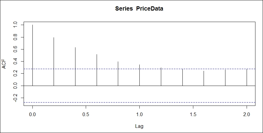
Figure 4.5: acf plot of price

Now let us plot pacf by executing the following code:

> pacf(PriceData, lag.max = 10) 

This generates the partial autocorrelation...

lock icon The rest of the chapter is locked
Register for a free Packt account to unlock a world of extra content!
A free Packt account unlocks extra newsletters, articles, discounted offers, and much more. Start advancing your knowledge today.
Unlock this book and the full library FREE for 7 days
Get unlimited access to 7000+ expert-authored eBooks and videos courses covering every tech area you can think of
Renews at $19.99/month. Cancel anytime
Banner background image