Search icon CANCEL
Subscription
0
Cart icon
Your Cart (0 item)
Close icon
You have no products in your basket yet
Save more on your purchases! discount-offer-chevron-icon
Savings automatically calculated. No voucher code required.
Arrow left icon
Explore Products
Best Sellers
New Releases
Books
Videos
Audiobooks
Learning Hub
Newsletter Hub
Free Learning
Arrow right icon
timer SALE ENDS IN
0 Days
:
00 Hours
:
00 Minutes
:
00 Seconds
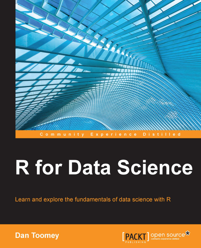
R for Data Science
R for Data Science

R for Data Science: Learn and explore the fundamentals of data science with R

eBook
$9.99 $32.99
Paperback
$54.99
Subscription
Free Trial
Renews at $19.99p/m

What do you get with Print?

Product feature icon Instant access to your digital eBook copy whilst your Print order is Shipped
Product feature icon Paperback book shipped to your preferred address
Product feature icon Download this book in EPUB and PDF formats
Product feature icon Access this title in our online reader with advanced features
Product feature icon DRM FREE - Read whenever, wherever and however you want
OR
Modal Close icon
Payment Processing...
tick Completed

Shipping Address

Billing Address

Shipping Methods
Table of content icon View table of contents Preview book icon Preview Book

R for Data Science

Chapter 1. Data Mining Patterns

A common use of data mining is to detect patterns or rules in data.

The points of interest are the non-obvious patterns that can only be detected using a large dataset. The detection of simpler patterns, such as market basket analysis for purchasing associations or timings, has been possible for some time. Our interest in R programming is in detecting unexpected associations that can lead to new opportunities.

Some patterns are sequential in nature, for example, predicting faults in systems based on past results that are, again, only obvious using large datasets. These will be explored in the next chapter.

This chapter discusses the use of R to discover patterns in datasets' various methods:

  • Cluster analysis: This is the process of examining your data and establishing groups of data points that are similar. Cluster analysis can be performed using several algorithms. The different algorithms focus on using different attributes of the data distribution, such as distance between points, density, or statistical ranges.
  • Anomaly detection: This is the process of looking at data that appears to be similar but shows differences or anomalies for certain attributes. Anomaly detection is used frequently in the field of law enforcement, fraud detection, and insurance claims.
  • Association rules: These are a set of decisions that can be made from your data. Here, we are looking for concrete steps so that if we find one data point, we can use a rule to determine whether another data point will likely exist. Rules are frequently used in market basket approaches. In data mining, we are looking for deeper, non-obvious rules that are present in the data.

Cluster analysis

Cluster analysis can be performed using a variety of algorithms; some of them are listed in the following table:

Type of model

How the model works

Connectivity

This model computes distance between points and organizes the points based on closeness.

Partitioning

This model partitions the data into clusters and associates each data point to a cluster. Most predominant is k-means.

Distribution Models

This model uses a statistical distribution to determine the clusters.

Density

This model determines closeness of data points to arrive at dense areas of distribution. The common use of DBSCAN is for tight concentrations or OPTICS for more sparse distributions.

Within an algorithm, there are finer levels of granularity as well, including:

  • Hard or soft clustering: It defines whether a data point can be part of more than one cluster.
  • Partitioning rules: Are rules that determine how to assign data points to different partitions. These rules are as follows:
    • Strict: This rule will check whether partitions include data points that are not close
    • Overlapping: This rule will check whether partitions overlap in any way
    • Hierarchical: This rule checks whether the partitions are stratified

In R programming, we have clustering tools for:

  • K-means clustering
  • K-medoids clustering
  • Hierarchical clustering
  • Expectation-maximization
  • Density estimation

K-means clustering

K-means clustering is a method of partitioning the dataset into k clusters. You need to predetermine the number of clusters you want to divide the dataset into. The k-means algorithm has the following steps:

  1. Select k random rows (centroids) from your data (you have a predetermined number of clusters to use).
  2. We are using Lloyd's algorithm (the default) to determine clusters.
  3. Assign each data point according to its closeness to a centroid.
  4. Recalculate each centroid as an average of all the points associated with it.
  5. Reassign each data point as closest to a centroid.
  6. Continue with steps 3 and 4 until data points are no longer assigned or you have looped some maximum number of times.

This is a heuristic algorithm, so it is a good idea to run the process several times. It will normally run quickly in R, as the work in each step is not difficult. The objective is to minimize the sum of squares by constant refining of the terms.

Predetermining the number of clusters may be problematic. Graphing the data (or its squares or the like) should present logical groupings for your data visually. You can determine group sizes by iterating through the steps to determine the cutoff for selection (we will use that later in this chapter). There are other R packages that will attempt to compute this as well. You should also verify the fit of the clusters selected upon completion.

Using an average (in step 3) shows that k-means does not work well with fairly sparse data or data with a larger number of outliers. Furthermore, there can be a problem if the cluster is not in a nice, linear shape. Graphical representation should prove whether your data fits this algorithm.

Usage

K-means clustering is performed in R programming with the kmeans function. The R programming usage of k-means clustering follows the convention given here (note that you can always determine the conventions for a function using the inline help function, for example, ?kmeans, to get this information):

kmeans(x, 
centers, 
iter.max = 10, 
nstart = 1,
algorithm = c("Hartigan-Wong",
                        "Lloyd",
                        "Forgy",
                        "MacQueen"), 
trace=FALSE)

The various parameters are explained in the following table:

Parameter

Description

x

This is the data matrix to be analyzed

centers

This is the number of clusters

iter.max

This is the maximum number of iterations (unless reassignment stops)

nstart

This is the number of random sets to use

algorithm

This can be of one of the following types: Hartigan-Wong, Lloyd, Forgy, or MacQueen algorithms

trace

This gives the present trace information as the algorithm progresses

Calling the kmeans function returns a kmeans object with the following properties:

Property

Description

cluster

This contains the cluster assignments

centers

This contains the cluster centers

totss

This gives the total sum of squares

withinss

This is the vector of within sum of squares, per cluster

tot.withinss

This contains the total (sum of withinss)

betweenss

This contains the between-cluster sum of squares

size

This contains the number of data points in each cluster

iter

This contains the number of iterations performed

ault

This contains the expert diagnostic

Example

First, generate a hundred pairs of random numbers in a normal distribution and assign it to the matrix x as follows:

>x <- rbind(matrix(rnorm(100, sd = 0.3), ncol = 2), 
                     matrix(rnorm(100, mean = 1, sd = 0.3), ncol = 2))

We can display the values we generate as follows:

>x
                [,1]          [,2]
  [1,]  0.4679569701  -0.269074028
  [2,] -0.5030944919  -0.393382748
  [3,] -0.3645075552  -0.304474590
…
 [98,]  1.1121388866   0.975150551
 [99,]  1.1818402912   1.512040138
[100,]  1.7643166039   1.339428999

The the resultant kmeans object values can be determined and displayed (using 10 clusters) as follows:

> fit <- kmeans(x,10)
> fit
K-means clustering with 10 clusters of sizes 4, 12, 10, 7, 13, 16, 8, 13, 8, 9
Cluster means:
          [,1]        [,2]
1   0.59611989  0.77213527
2   1.09064550  1.02456563
3  -0.01095292  0.41255130
4   0.07613688 -0.48816360
5   1.04043914  0.78864770
6   0.04167769 -0.05023832
7   0.47920281 -0.05528244
8   1.03305030  1.28488358
9   1.47791031  0.90185427
10 -0.28881626 -0.26002816
Clustering vector:
  [1]  7 10 10  6  7  6  3  3  7 10  4  7  4  7  6  7  6  6  4  3 10  4  3  6 10  6  6  3  6 10  3  6  4  3  6  3  6  6  6  7  3  4  6  7  6 10  4 10  3 10  5  2  9  2
 [55]  9  5  5  2  5  8  9  8  1  2  5  9  5  2  5  8  1  5  8  2  8  8  5  5  8  1  1  5  8  9  9  8  5  2  5  8  2  2  9  2  8  2  8  2  8  9
Within cluster sum of squares by cluster:
 [1] 0.09842712 0.23620192 0.47286373 0.30604945 0.21233870 0.47824982 0.36380678 0.58063931 0.67803464 0.28407093
 (between_SS / total_SS =  94.6 %)
Available components:
[1] "cluster"      "centers"      "totss"        "withinss"     "tot.withinss" "betweenss"    "size"         "iter"         "ifault"

If we look at the results, we find some interesting data points:

  • The Cluster means shows the breakdown of the means used for the cluster assignments.
  • The Clustering vector shows which cluster each of the 100 numbers was assigned to.
  • The Cluster sum of squares shows the totss value, as described in the output.
  • The percentage value is the betweenss value divided as a percentage of the totss value. At 94.6 percent, we have a very good fit.

We chose an arbitrary cluster size of 10, but we should verify that this is a good number to use. If we were to run the kmeans function a number of times using a range of cluster sizes, we would end up with a graph that looks like the one in the following example.

For example, if we ran the following code and recorded the results, the output will be as follows:

results <- matrix(nrow=14, ncol=2, dimnames=list(2:15,c("clusters","sumsquares")))
for(i in 2:15) {
  fit <- kmeans(x,i)
  results[i-1,1] <- i 
  results[i-1,2] <- fit$totss
}
plot(results)
Example

If the data were more distributed, there would be a clear demarcation about the maximum number of clusters, as further clustering will show no improvement in the sum of squares. However, since we used very smooth data for the test, the number of clusters could be allowed to increase.

Once your clusters have been determined, you should be able to gather a visual representation, as shown in the following plot:

Example

K-medoids clustering

K-medoids clustering is another method of determining the clusters in a dataset. A medoid is an entity of the dataset that represents the group to which it was inserted. K-means works with centroids, which are artificially created to represent a cluster. So, a medoid is actually part of the dataset. A centroid is a derived amount.

When partitioning around medoids, make sure that the following points are taken care of:

  • Each entity is assigned to only one cluster
  • Each entity is assigned to the medoid that defines its cluster
  • Exactly k clusters are defined

The algorithm has two phases with several steps:

  • Build phase: During the build phase, we come up with initial estimates for the clusters:
    1. Choose random k entities to become medoids (the k entities may be provided to the algorithm).
    2. Calculate the dissimilarity matrix (compute all the pairwise dissimilarities (distances) between observations in the dataset) so that we can find the distances.
    3. Assign every entity to the closest medoid.
  • Swap phase: In the swap phase, we fine-tune our initial estimates given the rough clusters determined in the build phase:
    1. Search each cluster for the entity that lowers the average dissimilarity coefficient the most and therefore makes it the medoid for the cluster.
    2. If any medoid has changed, start from step 3 of the build phase again.

Usage

K-medoid clustering is calculated in R programming with the pam function:

pam(x, k, diss, metric, medoids, stand, cluster.only, do.swap,   keep.diss, keep.data, trace.lev) 

The various parameters of the pam function are explained in the following table:

Parameter

Description

x

This is the data matrix or dissimilarity matrix (based on the diss flag)

k

This is the number of clusters, where 0 is less than k which is less than the number of entities

diss

The values are as follows:

  • FALSE if x is a matrix
  • TRUE if x is a dissimilarity matrix

metric

This is a string metric to be used to calculate the dissimilarity matrix. It can be of the following types:

  • euclidean for Euclidean distance
  • manhattan for Manhattan distance

medoids

If the NULL value is assigned, it means a set of medoids is to be developed. Otherwise, it is a set of initial medoids.

stand

If x is the data matrix, then measurements in x will be standardized before computing the dissimilarity matrix.

cluster.only

If the value set is TRUE, then only clustering will be computed and returned.

do.swap

This contains a Boolean value to decide whether swap should occur.

keep.diss

This contains a Boolean value to decide whether dissimilarity should be kept in the result.

keep.data

This contains a Boolean value to decide whether data should be kept in the result.

trace.lev

This contains an integer trace level for diagnostics, where 0 means no trace information.

The results returned from the pam function can be displayed, which is rather difficult to interpret, or the results can be plotted, which is intuitively more understandable.

Example

Using a simple set of data with two (visually) clear clusters as follows, as stored in a file named medoids.csv:

Object

x

y

1

1

10

2

2

11

3

1

10

4

2

12

5

1

4

6

3

5

7

2

6

8

2

5

9

3

6

Let's use the pam function on the medoids.csv file as follows:

# load pam function
> library(cluster)

#load the table from a file
> x <- read.table("medoids.csv", header=TRUE, sep=",")

#execute the pam algorithm with the dataset created for the example
> result <- pam(x, 2, FALSE, "euclidean")
Looking at the result directly we get:
> result
Medoids:
     ID Object x  y
[1,]  2      2 2 11
[2,]  7      7 2  6
Clustering vector:
[1] 1 1 1 1 2 2 2 2 2
Objective function:
   build     swap 
1.564722 1.564722 
Available components:
 [1] "medoids"    "id.med"     "clustering" "objective"  "isolation" 
[6] "clusinfo"   "silinfo"    "diss"       "call"       "data"

Evaluating the results we can see:

  • We specified the use of two medoids, and row 3 and 6 were chosen
  • The rows were clustered as presented in the clustering vector (as expected, about half in the first medoid and the rest in the other medoid)
  • The function did not change greatly from the build phase to the swap phase (looking at the Objective function values for build and swap of 1.56 versus 1.56)

Using a summary for a clearer picture, we see the following result:

> summary(result)
Medoids:
     ID Object x  y
[1,]  2      2 2 11
[2,]  7      7 2  6
Clustering vector:
[1] 1 1 1 1 2 2 2 2 2
Objective function:
   build     swap 
1.564722 1.564722 

Numerical information per cluster:
sizemax_dissav_diss diameter separation
[1,]    4 2.236068 1.425042 3.741657   5.744563
[2,]    5 3.000000 1.676466 4.898979   5.744563

Isolated clusters:
 L-clusters: character(0)
 L*-clusters: [1] 1 2

Silhouette plot information:
  cluster neighbor sil_width
2       1        2 0.7575089
3       1        2 0.6864544
1       1        2 0.6859661
4       1        2 0.6315196
8       2        1 0.7310922
7       2        1 0.6872724
6       2        1 0.6595811
9       2        1 0.6374808
5       2        1 0.5342637
Average silhouette width per cluster:
[1] 0.6903623 0.6499381
Average silhouette width of total data set:
[1] 0.6679044

36 dissimilarities, summarized :
   Min. 1st Qu.  Median    Mean 3rd Qu.    Max. 
 1.4142  2.3961  6.2445  5.2746  7.3822  9.1652 
Metric :  euclidean 
Number of objects : 9

Available components:
 [1] "medoids"    "id.med"     "clustering" "objective"  "isolation" 
 [6] "clusinfo"   "silinfo"    "diss"       "call"       "data"          

Tip

Downloading the example code

You can download the example code files from your account at http://www.packtpub.com for all the Packt Publishing books you have purchased. If you purchased this book elsewhere, you can visit http://www.packtpub.com/support and register to have the files e-mailed directly to you.

The summary presents more details on the medoids and how they were selected. However, note the dissimilarities as well.

Plotting the data, we can see the following output:

#plot a graphic showing the clusters and the medoids of each cluster
> plot(result$data, col = result$clustering)
Example

The resulting plot is as we expected it to be. It is good to see the data clearly broken into two medoids, both spatially and by color demarcation.

Hierarchical clustering

Hierarchical clustering is a method to ascertain clusters in a dataset that are in a hierarchy.

Using hierarchical clustering, we are attempting to create a hierarchy of clusters. There are two approaches of doing this:

  • Agglomerative (or bottom up): In this approach, each entity starts as its own cluster and pairs are merged as they move up the hierarchy
  • Divisive (or top down): In this approach, all entities are lumped into one cluster and are split as they are moved down the hierarchy

The resulting hierarchy is normally displayed using a tree/graph model of a dendogram.

Hierarchical clustering is performed in R programming with the hclust function.

Usage

The hclust function is called as follows:

hclust(d, method = "complete", members = NULL)

The various parameters of the hclust function are explained in the following table:

Parameter

Description

d

This is the matrix.

method

This is the agglomeration method to be used. This should be (a distinct abbreviation of) one of these methods: ward.D, ward.D2, single, complete, average (= UPGMA), mcquitty (= WPGMA), median (= WPGMC), or centroid (= UPGMC).

members

This could be NULL or d, the dissimilarity matrix.

Example

We start by generating some random data over a normal distribution using the following code:

> dat <- matrix(rnorm(100), nrow=10, ncol=10)

> dat
            [,1]       [,2]        [,3]        [,4]        [,5]       [,6]
 [1,]  1.4811953 -1.0882253 -0.47659922  0.22344983 -0.74227899  0.2835530
 [2,] -0.6414931 -1.0103688 -0.55213606 -0.48812235  1.41763706  0.8337524
 [3,]  0.2638638  0.2535630 -0.53310519  2.27778665 -0.09526058  1.9579652
[4,] -0.50307726 -0.3873578 -1.54407287 -0.1503834
Then, we calculate the hierarchical distribution for our data as follows:
> hc <- hclust(dist(dat))
> hc
Call:
hclust(d = dist(dat))

Cluster method   : complete 
Distance         : euclidean 
Number of objects: 10

The resulting data object is very uninformative. We can display the hierarchical cluster using a dendogram, as follows:

>plot(hc)
Example

The dendogram has the expected shape. I find these diagrams somewhat unclear, but if you go over them in detail, the inference will be as follows:

  • Reading the diagram in a top-down fashion, we see it has two distinct branches. The implication is that there are two groups that are distinctly different from one another. Within the two branches, we see 10 and 3 as distinctly different from the rest. Generally, it appears that we have determined there are an even group and an odd group, as expected.
  • Reading the diagram bottom up, we see closeness and similarity over a number of elements. This would be expected from a simple random distribution.

Expectation-maximization

Expectation-maximization (EM) is the process of estimating the parameters in a statistical model.

For a given model, we have the following parameters:

  • X: This is a set of observed data
  • Z: This is a set of missing values
  • T: This is a set of unknown parameters that we should apply to our model to predict Z

The steps to perform expectation-maximization are as follows:

  1. Initialize the unknown parameters (T) to random values.
  2. Compute the best missing values (Z) using the new parameter values.
  3. Use the best missing values (Z), which were just computed, to determine a better estimate for the unknown parameters (T).
  4. Iterate over steps 2 and 3 until we have a convergence.

This version of the algorithm produces hard parameter values (Z). In practice, soft values may be of interest where probabilities are assigned to various values of the parameters (Z). By hard values, I mean we are selecting specific Z values. We could instead use soft values where Z varies by some probability distribution.

We use EM in R programming with the Mclust function from the mclust library. The full description of Mclust is the normal mixture modeling fitted via EM algorithm for model-based clustering, classification, and density estimation, including Bayesian regularization.

Usage

The Mclust function is as follows:

Mclust(data, G = NULL, modelNames = NULL,
        prior = NULL, control = emControl(),
        initialization = NULL, warn = FALSE, ...)

The various parameters of the Mclust function are explained in the following table:

Parameter

Description

data

This contains the matrix.

G

This contains the vector of number of clusters to use to compute BIC. The default value is 1:9.

modelNames

This contains the vector of model names to use.

prior

This contains the optional conjugate prior for means.

control

This contains the list of control parameters for EM. The default value is List.

initialization

This contains NULL or a list of one or more of the following components:

  • hcPairs: This is used to merge pairs
  • subset: This is to be used during initialization
  • noise: This makes an initial guess at noise

warn

This contains which warnings are to be issued. Default is none.

List of model names

The Mclust function uses a model when trying to decide which items belong to a cluster. There are different model names for univariate, multivariate, and single component datasets. In each, the idea is to select a model that describes the data, for example, VII will be used for data that is spherically displaced with equal volume across each cluster.

Model

Type of dataset

Univariate mixture


E

equal variance (one-dimensional)

V

variable variance (one-dimensional)

Multivariate mixture


EII

spherical, equal volume

VII

spherical, unequal volume

EEI

diagonal, equal volume and shape

VEI

diagonal, varying volume, equal shape

EVI

diagonal, equal volume, varying shape

VVI

diagonal, varying volume and shape

EEE

ellipsoidal, equal volume, shape, and orientation

EEV

ellipsoidal, equal volume and equal shape

VEV

ellipsoidal, equal shape

VVV

ellipsoidal, varying volume, shape, and orientation

Single component


X

univariate normal

XII

spherical multivariate normal

XXI

diagonal multivariate normal

XXX

ellipsoidal multivariate normal

Example

First, we must load the library that contains the mclust function (we may need to install it in the local environment) as follows:

> install.packages("mclust")
> library(mclust)

We will be using the iris data in this example, as shown here:

> data <- read.csv("http://archive.ics.uci.edu/ml/machine-learning-databases/iris/iris.data")

Now, we can compute the best fit via EM (note capitalization of Mclust) as follows:

> fit <- Mclust(data)

We can display our results as follows:

> fit
'Mclust' model object:
 best model: ellipsoidal, equal shape (VEV) with 2 components

> summary(fit)
----------------------------------------------------
Gaussian finite mixture model fitted by EM algorithm 
----------------------------------------------------
Mclust VEV (ellipsoidal, equal shape) model with 2 components:

 log.likelihood   n df       BIC       ICL
      -121.1459 149 37 -427.4378 -427.4385

Clustering table:
  1   2 
 49 100

Simple display of the fit data object doesn't tell us very much, it shows just what was used to compute the density of the dataset.

The summary command presents more detailed information about the results, as listed here:

  • log.likelihood (-121): This is the log likelihood of the BIC value
  • n (149): This is the number of data points
  • df (37): This is the distribution
  • BIC (-427): This is the Bayesian information criteria; this is an optimal value
  • ICL (-427): Integrated Complete Data Likelihood—a classification version of the BIC. As we have the same value for ICL and BIC we classified the data points.

We can plot the results for a visual verification as follows:

> plot(fit)

You will notice that the plot command for EM produces the following four plots (as shown in the graph):

  • The BIC values used for choosing the number of clusters
  • A plot of the clustering
  • A plot of the classification uncertainty
  • The orbital plot of clusters

The following graph depicts the plot of density.

The first plot gives a depiction of the BIC ranges versus the number of components by different model names; in this case, we should probably not use VEV, for example:

Example

This second plot shows the comparison of using each of the components of the data feed against every other component of the data feed to determine the clustering that would result. The idea is to select the components that give you the best clustering of your data. This is one of those cases where your familiarity with the data is key to selecting the appropriate data points for clustering.

In this case, I think selecting X5.1 and X1.4 yield the tightest clusters, as shown in the following graph:

.

Example

The third plot gives another iteration of the clustering affects of the different choices highlighting the main cluster by eliminating any points from the plot that would be applied to the main cluster, as shown here:

Example

The final, fourth plot gives an orbital view of each of the clusters giving a highlight display of where the points might appear relative to the center of each cluster, as shown here:

Example

Density estimation

Density estimation is the process of estimating the probability density function of a population given in an observation set. The density estimation process takes your observations, disperses them across a number of data points, runs a FF transform to determine a kernel, and then runs a linear approximation to estimate density.

Density estimation produces an estimate for the unobservable population distribution function. Some approaches that are used to produce the density estimation are as follows:

  • Parzen windows: In this approach, the observations are placed in a window and density estimates are made based on proximity
  • Vector quantization: This approach lets you model the probability density functions as per the distribution of observations
  • Histograms: With a histogram, you get a nice visual showing density (size of the bars); the number of bins chosen while developing the histogram decide your density outcome

Density estimation is performed via the density function in R programming. Other functions for density evaluation in R are:

Function

Description

DBSCAN

This function determines clustering for fixed point clusters

OPTICS

This function determines clustering for wide distribution clusters

Usage

The density function is invoked as follows:

density(x, bw = "nrd0", adjust = 1,
        kernel = c("gaussian", "epanechnikov",
                   "rectangular",
                   "triangular", "biweight",
                   "cosine", "optcosine"),
        weights = NULL, window = kernel, width,
        give.Rkern = FALSE,
        n = 512, from, to, na.rm = FALSE, ...) 

The various parameters of the density function are explained in the following table:

Parameter

Description

x

This is the matrix.

bw

This is the smoothing bandwidth to be used.

adjust

This is the multiplier to adjust bandwidth.

kernel

This is the smoother kernel to be used. It must be one of the following kernels:

  • gaussian
  • rectangular
  • triangular
  • epanechnikov
  • biweight
  • cosine
  • optcosine

weights

This is a vector of observation weights with same length as x.

window

This is the kernel used.

width

This is the S compatibility parameter.

give.Rkern

If the value of this parameter is TRUE, no density is estimated.

N

This is the number of density points to estimate.

from, to

These are the left and right-most points to use.

na.rm

If the value of this parameter is TRUE, missing values are removed.

The available bandwidths can be found using the following commands:

bw.nrd0(x)

bw.nrd(x)

bw.ucv(x, nb = 1000, lower = 0.1 * hmax, upper = hmax, tol = 0.1 * lower)

bw.bcv(x, nb = 1000, lower = 0.1 * hmax, upper = hmax, tol = 0.1 * lower)

bw.SJ(x, nb = 1000, lower = 0.1 * hmax, upper = hmax, method = 
  c("ste", "dpi"), tol = 0.1 * lower)

The various parameters of the bw function are explained in the following table:

Parameter

Description

x

This is the dataset

nb

This is the number of bins

lower, upper

This is the range of bandwidth which is to be minimized

method

The ste method is used to solve the equation or the dpi method is used for direct plugin

tol

This is the convergence tolerance for ste

Example

We can use the iris dataset as follows:

> data <- read.csv("http://archive.ics.uci.edu/ml/machine-learning-databases/iris/iris.data")
The density of the X5.1 series (sepal length) can be computed as follows:
> d <- density(data$X5.1)
> d
Call:
density.default(x = data$X5.1)
Data: data$X5.1 (149 obs.);  Bandwidth 'bw' = 0.2741
       x               y            
 Min.:3.478   Min.   :0.0001504  
 1st Qu.:4.789   1st Qu.:0.0342542  
 Median :6.100   Median :0.1538908  
 Mean   :6.100   Mean   :0.1904755  
 3rd Qu.:7.411   3rd Qu.:0.3765078  
 Max.   :8.722   Max.   :0.3987472  

We can plot the density values as follows:

> plot(d)
Example

The plot shows most of the data occurring between 5 and 7. So, sepal length averages at just under 6.

Anomaly detection

We can use R programming to detect anomalies in a dataset. Anomaly detection can be used in a number of different areas, such as intrusion detection, fraud detection, system health, and so on. In R programming, these are called outliers. R programming allows the detection of outliers in a number of ways, as listed here:

  • Statistical tests
  • Depth-based approaches
  • Deviation-based approaches
  • Distance-based approaches
  • Density-based approaches
  • High-dimensional approaches

Show outliers

R programming has a function to display outliers: identify (in boxplot).

The boxplot function produces a box-and-whisker plot (see following graph). The boxplot function has a number of graphics options. For this example, we do not need to set any.

The identify function is a convenient method for marking points in a scatter plot. In R programming, box plot is a type of scatter plot.

Example

In this example, we need to generate a 100 random numbers and then plot the points in boxes.

Then, we mark the first outlier with it's identifier as follows:

> y <- rnorm(100)
> boxplot(y)
> identify(rep(1, length(y)), y, labels = seq_along(y))
Example

Note

Notice the 0 next to the outlier in the graph.

Example

The boxplot function automatically computes the outliers for a set as well.

First, we will generate a 100 random numbers as follows (note that this data is randomly generated, so your results may not be the same):

> x <- rnorm(100)

We can have a look at the summary information on the set using the following code:

> summary(x)
    Min.  1st Qu.   Median     Mean  3rd Qu.     Max. 
-2.12000 -0.74790 -0.20060 -0.01711  0.49930  2.43200

Now, we can display the outliers using the following code:

> boxplot.stats(x)$out
[1] 2.420850 2.432033

The following code will graph the set and highlight the outliers:

> boxplot(x)
Example

Note

Notice the 0 next to the outlier in the graph.

We can generate a box plot of more familiar data showing the same issue with outliers using the built-in data for cars, as follows:

boxplot(mpg~cyl,data=mtcars, xlab="Cylinders", ylab="MPG")
Example

Another anomaly detection example

We can also use box plot's outlier detection when we have two dimensions. Note that we are forcing the issue by using a union of the outliers in x and y rather than an intersection. The point of the example is to display such points. The code is as follows:

> x <- rnorm(1000)
> y <- rnorm(1000)
> f <- data.frame(x,y)
> a <- boxplot.stats(x)$out
> b <- boxplot.stats(y)$out
> list <- union(a,b)
> plot(f)
> px <- f[f$x %in% a,]
> py <- f[f$y %in% b,]
> p <- rbind(px,py)
> par(new=TRUE)
> plot(p$x, p$y,cex=2,col=2)
Another anomaly detection example

While R did what we asked, the plot does not look right. We completely fabricated the data; in a real use case, you would need to use your domain expertise to determine whether these outliers were correct or not.

Calculating anomalies

Given the variety of what constitutes an anomaly, R programming has a mechanism that gives you complete control over it: write your own function that can be used to make a decision.

Usage

We can use the name function to create our own anomaly as shown here:

name <- function(parameters,…) {
  # determine what constitutes an anomaly
  return(df)
}

Here, the parameters are the values we need to use in the function. I am assuming we return a data frame from the function. The function could do anything.

Example 1

We will be using the iris data in this example, as shown here:

> data <- read.csv("http://archive.ics.uci.edu/ml/machine-learning-databases/iris/iris.data")

If we decide an anomaly is present when sepal is under 4.5 or over 7.5, we could use a function as shown here:

> outliers <- function(data, low, high) {
>  outs <- subset(data, data$X5.1 < low | data$X5.1 > high)
>  return(outs)
>}

Then, we will get the following output:

> outliers(data, 4.5, 7.5)
    X5.1 X3.5 X1.4 X0.2    Iris.setosa
8    4.4  2.9  1.4  0.2    Iris-setosa
13   4.3  3.0  1.1  0.1    Iris-setosa
38   4.4  3.0  1.3  0.2    Iris-setosa
42   4.4  3.2  1.3  0.2    Iris-setosa
105  7.6  3.0  6.6  2.1 Iris-virginica
117  7.7  3.8  6.7  2.2 Iris-virginica
118  7.7  2.6  6.9  2.3 Iris-virginica
122  7.7  2.8  6.7  2.0 Iris-virginica
131  7.9  3.8  6.4  2.0 Iris-virginica
135  7.7  3.0  6.1  2.3 Iris-virginica

This gives us the flexibility of making slight adjustments to our criteria by passing different parameter values to the function in order to achieve the desired results.

Example 2

Another popular package is DMwR. It contains the lofactor function that can also be used to locate outliers. The DMwR package can be installed using the following command:

> install.packages("DMwR")
> library(DMwR)

We need to remove the species column from the data, as it is categorical against it data. This can be done by using the following command:

> nospecies <- data[,1:4]

Now, we determine the outliers in the frame:

> scores <- lofactor(nospecies, k=3)

Next, we take a look at their distribution:

> plot(density(scores))
Example 2

One point of interest is if there is some close equality amongst several of the outliers (that is, density of about 4).

Association rules

Association rules describe associations between two datasets. This is most commonly used in market basket analysis. Given a set of transactions with multiple, different items per transaction (shopping bag), how can the item sales be associated? The most common associations are as follows:

  • Support: This is the percentage of transactions that contain A and B.
  • Confidence: This is the percentage (of time that rule is correct) of cases containing A that also contain B.
  • Lift: This is the ratio of confidence to the percentage of cases containing B. Please note that if lift is 1, then A and B are independent.

Mine for associations

The most widely used tool in R from association rules is apriori.

Usage

The apriori rules library can be called as follows:

apriori(data, parameter = NULL, appearance = NULL, control = NULL)

The various parameters of the apriori library are explained in the following table:

Parameter

Description

data

This is the transaction data.

parameter

This stores the default behavior to mine, with support as 0.1, confidence as 0.8, and maxlen as 10. You can change parameter values accordingly.

appearance

This is used to restrict items that appear in rules.

control

This is used to adjust the performance of the algorithm used.

Example

You will need to load the apriori rules library as follows:

> install.packages("arules")
> library(arules)

The market basket data can be loaded as follows:

> data <- read.csv("http://www.salemmarafi.com/wp-content/uploads/2014/03/groceries.csv")

Then, we can generate rules from the data as follows:

> rules <- apriori(data) 

parameter specification:
confidenceminvalsmaxaremavaloriginalSupport support minlenmaxlen target
        0.8    0.1    1 none FALSE            TRUE     0.1      1     10  rules
   ext
 FALSE

algorithmic control:
 filter tree heap memopt load sort verbose
    0.1 TRUE TRUE  FALSE TRUE    2    TRUE

apriori - find association rules with the apriori algorithm
version 4.21 (2004.05.09)        (c) 1996-2004   Christian Borgelt
set item appearances ...[0 item(s)] done [0.00s].
set transactions ...[655 item(s), 15295 transaction(s)] done [0.00s].
sorting and recoding items ... [3 item(s)] done [0.00s].
creating transaction tree ... done [0.00s].
checking subsets of size 1 2 3 done [0.00s].
writing ... [5 rule(s)] done [0.00s].
creating S4 object  ... done [0.00s].

There are several points to highlight in the results:

  • As you can see from the display, we are using the default settings (confidence 0.8, and so on)
  • We found 15,000 transactions for three items (picked from the 655 total items available)
  • We generated five rules

We can examine the rules that were generated as follows:

> rules

set of 5 rules 
> inspect(rules)

lhsrhs              support confidence     lift
1 {semi.finished.bread=} => {margarine=}   0.2278522          1 2.501226
2 {semi.finished.bread=} => {ready.soups=} 0.2278522          1 1.861385
3 {margarine=}           => {ready.soups=} 0.3998039          1 1.861385
4 {semi.finished.bread=,                                                
   margarine=}           => {ready.soups=} 0.2278522          1 1.861385
5 {semi.finished.bread=,                                                
   ready.soups=}         => {margarine=}   0.2278522          1 2.501226

The code has been slightly reformatted for readability.

Looking over the rules, there is a clear connection between buying bread, soup, and margarine—at least in the market where and when the data was gathered.

If we change the parameters (thresholds) used in the calculation, we get a different set of rules. For example, check the following code:

> rules <- apriori(data, parameter = list(supp = 0.001, conf = 0.8))

This code generates over 500 rules, but they have questionable meaning as we now have the rules with 0.001 confidence.

Questions

Factual

  • How do you decide whether to use kmeans or kdemoids?
  • What is the significance of the boxplot layout? Why does it look that way?
  • Describe the underlying data produced in the outliers for the iris data, given the density plot.
  • What are the extract rules for other items in the market dataset?

When, how, and why?

  • What is the risk of not vetting the outliers that are detected for the specific domain? Shouldn't the calculation always work?
  • Why do we need to exclude the iris category column from the outlier detection algorithm? Can it be used in some way when determining outliers?
  • Can you come up with a scenario where the market basket data and rules we generated were not applicable to the store you are working with?

Challenges

  • I found it difficult to develop test data for outliers in two dimensions that both occurred in the same instance using random data. Can you develop a test that would always have several outliers in at least two dimensions that occur in the same instance?
  • There is a good dataset on the Internet regarding passenger data on the Titanic. Generate the rules regarding the possible survival of the passengers.

Summary

In this chapter, we discussed cluster analysis, anomaly detection, and association rules. In cluster analysis, we use k-means clustering, k-medoids clustering, hierarchical clustering, expectation-maximization, and density estimation. In anomaly detection, we found outliers using built-in R functions and developed our own specialized R function. For association rules, we used the apriori package to determine the associations amongst datasets.

In the next chapter, we will cover data mining for sequences.

Left arrow icon Right arrow icon

Description

If you are a data analyst who has a firm grip on some advanced data analysis techniques and wants to learn how to leverage the features of R, this is the book for you. You should have some basic knowledge of the R language and should know about some data science topics.

What you will learn

  • Develop, execute, and modify R scripts
  • Learn how to use different data mining sequences
  • Find out how to organize your data effectively
  • Produce highquality data visualizations
  • Get to grips with a number of approaches to the statistical analysis of data
  • Learn how to cultivate a strategic approach to your data to use the right tools, models and visualizations to get the job done
Estimated delivery fee Deliver to Indonesia

Standard delivery 10 - 13 business days

$12.95

Premium delivery 5 - 8 business days

$45.95
(Includes tracking information)

Product Details

Country selected
Publication date, Length, Edition, Language, ISBN-13
Publication date : Dec 24, 2014
Length: 364 pages
Edition : 1st
Language : English
ISBN-13 : 9781784390860
Category :
Languages :
Concepts :

What do you get with Print?

Product feature icon Instant access to your digital eBook copy whilst your Print order is Shipped
Product feature icon Paperback book shipped to your preferred address
Product feature icon Download this book in EPUB and PDF formats
Product feature icon Access this title in our online reader with advanced features
Product feature icon DRM FREE - Read whenever, wherever and however you want
OR
Modal Close icon
Payment Processing...
tick Completed

Shipping Address

Billing Address

Shipping Methods
Estimated delivery fee Deliver to Indonesia

Standard delivery 10 - 13 business days

$12.95

Premium delivery 5 - 8 business days

$45.95
(Includes tracking information)

Product Details

Publication date : Dec 24, 2014
Length: 364 pages
Edition : 1st
Language : English
ISBN-13 : 9781784390860
Category :
Languages :
Concepts :

Packt Subscriptions

See our plans and pricing
Modal Close icon
$19.99 billed monthly
Feature tick icon Unlimited access to Packt's library of 7,000+ practical books and videos
Feature tick icon Constantly refreshed with 50+ new titles a month
Feature tick icon Exclusive Early access to books as they're written
Feature tick icon Solve problems while you work with advanced search and reference features
Feature tick icon Offline reading on the mobile app
Feature tick icon Simple pricing, no contract
$199.99 billed annually
Feature tick icon Unlimited access to Packt's library of 7,000+ practical books and videos
Feature tick icon Constantly refreshed with 50+ new titles a month
Feature tick icon Exclusive Early access to books as they're written
Feature tick icon Solve problems while you work with advanced search and reference features
Feature tick icon Offline reading on the mobile app
Feature tick icon Choose a DRM-free eBook or Video every month to keep
Feature tick icon PLUS own as many other DRM-free eBooks or Videos as you like for just $5 each
Feature tick icon Exclusive print discounts
$279.99 billed in 18 months
Feature tick icon Unlimited access to Packt's library of 7,000+ practical books and videos
Feature tick icon Constantly refreshed with 50+ new titles a month
Feature tick icon Exclusive Early access to books as they're written
Feature tick icon Solve problems while you work with advanced search and reference features
Feature tick icon Offline reading on the mobile app
Feature tick icon Choose a DRM-free eBook or Video every month to keep
Feature tick icon PLUS own as many other DRM-free eBooks or Videos as you like for just $5 each
Feature tick icon Exclusive print discounts

Frequently bought together


Stars icon
Total $ 153.97
Python Data Analysis
$54.99
R for Data Science
$54.99
Python Data Science Essentials
$43.99
Total $ 153.97 Stars icon
Banner background image

Table of Contents

13 Chapters
1. Data Mining Patterns Chevron down icon Chevron up icon
2. Data Mining Sequences Chevron down icon Chevron up icon
3. Text Mining Chevron down icon Chevron up icon
4. Data Analysis – Regression Analysis Chevron down icon Chevron up icon
5. Data Analysis – Correlation Chevron down icon Chevron up icon
6. Data Analysis – Clustering Chevron down icon Chevron up icon
7. Data Visualization – R Graphics Chevron down icon Chevron up icon
8. Data Visualization – Plotting Chevron down icon Chevron up icon
9. Data Visualization – 3D Chevron down icon Chevron up icon
10. Machine Learning in Action Chevron down icon Chevron up icon
11. Predicting Events with Machine Learning Chevron down icon Chevron up icon
12. Supervised and Unsupervised Learning Chevron down icon Chevron up icon
Index Chevron down icon Chevron up icon

Customer reviews

Rating distribution
Full star icon Full star icon Full star icon Half star icon Empty star icon 3.4
(5 Ratings)
5 star 60%
4 star 0%
3 star 0%
2 star 0%
1 star 40%
Luis Jose Muãiz Rascado Apr 23, 2016
Full star icon Full star icon Full star icon Full star icon Full star icon 5
excelent issue!!!!
Amazon Verified review Amazon
Ketan Jan 29, 2015
Full star icon Full star icon Full star icon Full star icon Full star icon 5
Recently completed reading this book on my kindle! To be honest, I judged the book by its cover when it says “Learn and explore the fundamentals of data science with R,” I believed it. This book covers various cluster analysis, data mining, regression and graphics and much more. The highlight of the book for me was its section “Machine Learning in Action.”Though I will be going through the book again to find out details I must have missed, but on an overview, I can say that this will be an important book in my kindle library. I realised it is not wrong to judge the book by its cover.A must read for all data scientists!
Amazon Verified review Amazon
Akshul Agarwal Jan 29, 2015
Full star icon Full star icon Full star icon Full star icon Full star icon 5
I recently purchased two books from Packt Publishing, R Object Oriented Programming and this one, R for data sciences. The authors seem to have a thorough understanding of the topics and moreover have a knack for keeping the content so simplistic that even beginners would eventually find their path to understand the topic with ease. As the description suggests, the purpose of the book is to explore the core topics that a person interested in R would want to read about. The content of the book was indeed what I have been looking for. This book draws from an extensive assortment of data sources and works on the data using very easily available R functions and packages over the web.
Amazon Verified review Amazon
Amazon Customer Oct 19, 2017
Full star icon Empty star icon Empty star icon Empty star icon Empty star icon 1
Terrible book. There are topics that are presented multiple times on the book, independently. It limits itself to a copy paste of the input and output parameters of some data science methods, without giving any explanations and with multiple errors.
Amazon Verified review Amazon
Logan Sep 02, 2015
Full star icon Empty star icon Empty star icon Empty star icon Empty star icon 1
"From the results, we can see R-squared of close to 0 and p-value almost 1; this is a very good fit." (p. 309)This is a direct quote from this book. When you can't understand the most basic aspect of linear regression you have no business selling a book on "data science." Run away, run very far away and download something like the free Introduction to Statistical Learning if you really want to learn R and the basics of data science.
Amazon Verified review Amazon
Get free access to Packt library with over 7500+ books and video courses for 7 days!
Start Free Trial

FAQs

What is the delivery time and cost of print book? Chevron down icon Chevron up icon

Shipping Details

USA:

'

Economy: Delivery to most addresses in the US within 10-15 business days

Premium: Trackable Delivery to most addresses in the US within 3-8 business days

UK:

Economy: Delivery to most addresses in the U.K. within 7-9 business days.
Shipments are not trackable

Premium: Trackable delivery to most addresses in the U.K. within 3-4 business days!
Add one extra business day for deliveries to Northern Ireland and Scottish Highlands and islands

EU:

Premium: Trackable delivery to most EU destinations within 4-9 business days.

Australia:

Economy: Can deliver to P. O. Boxes and private residences.
Trackable service with delivery to addresses in Australia only.
Delivery time ranges from 7-9 business days for VIC and 8-10 business days for Interstate metro
Delivery time is up to 15 business days for remote areas of WA, NT & QLD.

Premium: Delivery to addresses in Australia only
Trackable delivery to most P. O. Boxes and private residences in Australia within 4-5 days based on the distance to a destination following dispatch.

India:

Premium: Delivery to most Indian addresses within 5-6 business days

Rest of the World:

Premium: Countries in the American continent: Trackable delivery to most countries within 4-7 business days

Asia:

Premium: Delivery to most Asian addresses within 5-9 business days

Disclaimer:
All orders received before 5 PM U.K time would start printing from the next business day. So the estimated delivery times start from the next day as well. Orders received after 5 PM U.K time (in our internal systems) on a business day or anytime on the weekend will begin printing the second to next business day. For example, an order placed at 11 AM today will begin printing tomorrow, whereas an order placed at 9 PM tonight will begin printing the day after tomorrow.


Unfortunately, due to several restrictions, we are unable to ship to the following countries:

  1. Afghanistan
  2. American Samoa
  3. Belarus
  4. Brunei Darussalam
  5. Central African Republic
  6. The Democratic Republic of Congo
  7. Eritrea
  8. Guinea-bissau
  9. Iran
  10. Lebanon
  11. Libiya Arab Jamahriya
  12. Somalia
  13. Sudan
  14. Russian Federation
  15. Syrian Arab Republic
  16. Ukraine
  17. Venezuela
What is custom duty/charge? Chevron down icon Chevron up icon

Customs duty are charges levied on goods when they cross international borders. It is a tax that is imposed on imported goods. These duties are charged by special authorities and bodies created by local governments and are meant to protect local industries, economies, and businesses.

Do I have to pay customs charges for the print book order? Chevron down icon Chevron up icon

The orders shipped to the countries that are listed under EU27 will not bear custom charges. They are paid by Packt as part of the order.

List of EU27 countries: www.gov.uk/eu-eea:

A custom duty or localized taxes may be applicable on the shipment and would be charged by the recipient country outside of the EU27 which should be paid by the customer and these duties are not included in the shipping charges been charged on the order.

How do I know my custom duty charges? Chevron down icon Chevron up icon

The amount of duty payable varies greatly depending on the imported goods, the country of origin and several other factors like the total invoice amount or dimensions like weight, and other such criteria applicable in your country.

For example:

  • If you live in Mexico, and the declared value of your ordered items is over $ 50, for you to receive a package, you will have to pay additional import tax of 19% which will be $ 9.50 to the courier service.
  • Whereas if you live in Turkey, and the declared value of your ordered items is over € 22, for you to receive a package, you will have to pay additional import tax of 18% which will be € 3.96 to the courier service.
How can I cancel my order? Chevron down icon Chevron up icon

Cancellation Policy for Published Printed Books:

You can cancel any order within 1 hour of placing the order. Simply contact customercare@packt.com with your order details or payment transaction id. If your order has already started the shipment process, we will do our best to stop it. However, if it is already on the way to you then when you receive it, you can contact us at customercare@packt.com using the returns and refund process.

Please understand that Packt Publishing cannot provide refunds or cancel any order except for the cases described in our Return Policy (i.e. Packt Publishing agrees to replace your printed book because it arrives damaged or material defect in book), Packt Publishing will not accept returns.

What is your returns and refunds policy? Chevron down icon Chevron up icon

Return Policy:

We want you to be happy with your purchase from Packtpub.com. We will not hassle you with returning print books to us. If the print book you receive from us is incorrect, damaged, doesn't work or is unacceptably late, please contact Customer Relations Team on customercare@packt.com with the order number and issue details as explained below:

  1. If you ordered (eBook, Video or Print Book) incorrectly or accidentally, please contact Customer Relations Team on customercare@packt.com within one hour of placing the order and we will replace/refund you the item cost.
  2. Sadly, if your eBook or Video file is faulty or a fault occurs during the eBook or Video being made available to you, i.e. during download then you should contact Customer Relations Team within 14 days of purchase on customercare@packt.com who will be able to resolve this issue for you.
  3. You will have a choice of replacement or refund of the problem items.(damaged, defective or incorrect)
  4. Once Customer Care Team confirms that you will be refunded, you should receive the refund within 10 to 12 working days.
  5. If you are only requesting a refund of one book from a multiple order, then we will refund you the appropriate single item.
  6. Where the items were shipped under a free shipping offer, there will be no shipping costs to refund.

On the off chance your printed book arrives damaged, with book material defect, contact our Customer Relation Team on customercare@packt.com within 14 days of receipt of the book with appropriate evidence of damage and we will work with you to secure a replacement copy, if necessary. Please note that each printed book you order from us is individually made by Packt's professional book-printing partner which is on a print-on-demand basis.

What tax is charged? Chevron down icon Chevron up icon

Currently, no tax is charged on the purchase of any print book (subject to change based on the laws and regulations). A localized VAT fee is charged only to our European and UK customers on eBooks, Video and subscriptions that they buy. GST is charged to Indian customers for eBooks and video purchases.

What payment methods can I use? Chevron down icon Chevron up icon

You can pay with the following card types:

  1. Visa Debit
  2. Visa Credit
  3. MasterCard
  4. PayPal
What is the delivery time and cost of print books? Chevron down icon Chevron up icon

Shipping Details

USA:

'

Economy: Delivery to most addresses in the US within 10-15 business days

Premium: Trackable Delivery to most addresses in the US within 3-8 business days

UK:

Economy: Delivery to most addresses in the U.K. within 7-9 business days.
Shipments are not trackable

Premium: Trackable delivery to most addresses in the U.K. within 3-4 business days!
Add one extra business day for deliveries to Northern Ireland and Scottish Highlands and islands

EU:

Premium: Trackable delivery to most EU destinations within 4-9 business days.

Australia:

Economy: Can deliver to P. O. Boxes and private residences.
Trackable service with delivery to addresses in Australia only.
Delivery time ranges from 7-9 business days for VIC and 8-10 business days for Interstate metro
Delivery time is up to 15 business days for remote areas of WA, NT & QLD.

Premium: Delivery to addresses in Australia only
Trackable delivery to most P. O. Boxes and private residences in Australia within 4-5 days based on the distance to a destination following dispatch.

India:

Premium: Delivery to most Indian addresses within 5-6 business days

Rest of the World:

Premium: Countries in the American continent: Trackable delivery to most countries within 4-7 business days

Asia:

Premium: Delivery to most Asian addresses within 5-9 business days

Disclaimer:
All orders received before 5 PM U.K time would start printing from the next business day. So the estimated delivery times start from the next day as well. Orders received after 5 PM U.K time (in our internal systems) on a business day or anytime on the weekend will begin printing the second to next business day. For example, an order placed at 11 AM today will begin printing tomorrow, whereas an order placed at 9 PM tonight will begin printing the day after tomorrow.


Unfortunately, due to several restrictions, we are unable to ship to the following countries:

  1. Afghanistan
  2. American Samoa
  3. Belarus
  4. Brunei Darussalam
  5. Central African Republic
  6. The Democratic Republic of Congo
  7. Eritrea
  8. Guinea-bissau
  9. Iran
  10. Lebanon
  11. Libiya Arab Jamahriya
  12. Somalia
  13. Sudan
  14. Russian Federation
  15. Syrian Arab Republic
  16. Ukraine
  17. Venezuela