Second use case – simple linear regression
The objective of this example is to show how to log a metric in Comet. In detail, we set up an experiment that calculates the different values of Mean Squared Error (MSE) produced by fitting a linear regression model with different training sets. Every training set is derived from the same original dataset, by specifying a different seed.
You can download the full code of this example from the official GitHub repository of the book, available at the following link: https://github.com/PacktPublishing/Comet-for-Data-Science/tree/main/01.
We use the scikit-learn Python package to implement a linear regression model. For this use case, we will use the diabetes dataset, provided by scikit-learn.
We organize the experiment in three steps:
- Initialize the context.
- Define, fit, and evaluate the model.
- Show results in Comet.
Let's start with the first step: initializing the context.
Initializing the context
Firstly, we create a .comet.config file in our working directory, as explained in the Getting started with workspaces, projects, experiments, and panels, in the Experiment section.
As the first statement of our code, we create a Comet experiment, as follows:
from comet-ml import Experiment
experiment = Experiment()
Now, we load the diabetes dataset, provided by scikit-learn, as follows:
from sklearn.datasets import load_diabetes
diabetes = load_diabetes()
X = diabetes.data
y = diabetes.target
We load the dataset and stored data and target in X and y variables, respectively.
Our context is now ready, so we can move on to the second part of our experiment: defining, fitting, and evaluating the model.
Defining, fitting, and evaluating the model
Let's start with the imports:
- Firstly, we import all the libraries and functions that we will use:
import numpy as np
from sklearn.model_selection import train_test_split
from sklearn.linear_model import LinearRegression
from sklearn.metrics import mean_squared_error
We import NumPy, which we will use to build the array of different seeds, and other scikit-learn classes and methods used for the modeling phase.
- We set the seeds to test, as follows:
n = 100
seed_list = np.arange(0, n+1, step = 5)
We define 20 different seeds, ranging from 0 to 100, with a step of 5. Thus, we have 0, 5, 10, 15 … 95, 100.
- For each seed, we extract a different training and test set, which we use to train the same model, calculate the MSE, and log it in Comet, using the following code:
for seed in seed_list:
    X_train, X_test, y_train, y_test = train_test_split(X, y, test_size=0.20, random_state=seed)
    model = LinearRegression()
    model.fit(X_train,y_train)
    y_pred = model.predict(X_test)
    mse = mean_squared_error(y_test,y_pred)
    experiment.log_metric("MSE", mse, step=seed)
In the previous code, firstly we split the dataset into training and test sets, using the current seed. We reserve 20% of the data for the test set and the remaining 80% for the training set. Then, we build the linear regression model, we fit it (model.fit()), and we predict the next values for the test set (model.predict()). We also calculate MSE through the mean_squared_error() function. Finally, we log the metric in Comet through the log_metric() method. The log_metric() method receives the metric name as the first parameter and the metric value as the second parameter. We also specify the step for the metric that corresponds to the seed, in our case.
Now, we can launch the code and see the results in Comet.
Showing results in Comet
To see the results in Comet, we perform the following steps:
- Open your Comet project.
- Select Experiments from the top menu.
- The dashboard shows a list of all the experiments. In our case, there is just one experiment.
- Click on the experiment name, in the first cell on the left. Since we have not set the experiment name, Comet has set the experiment name for us. Comet shows a dashboard with all the experiment details.
In our experiment, we can see some results in three different sections: Charts, Metrics, and System Metrics.
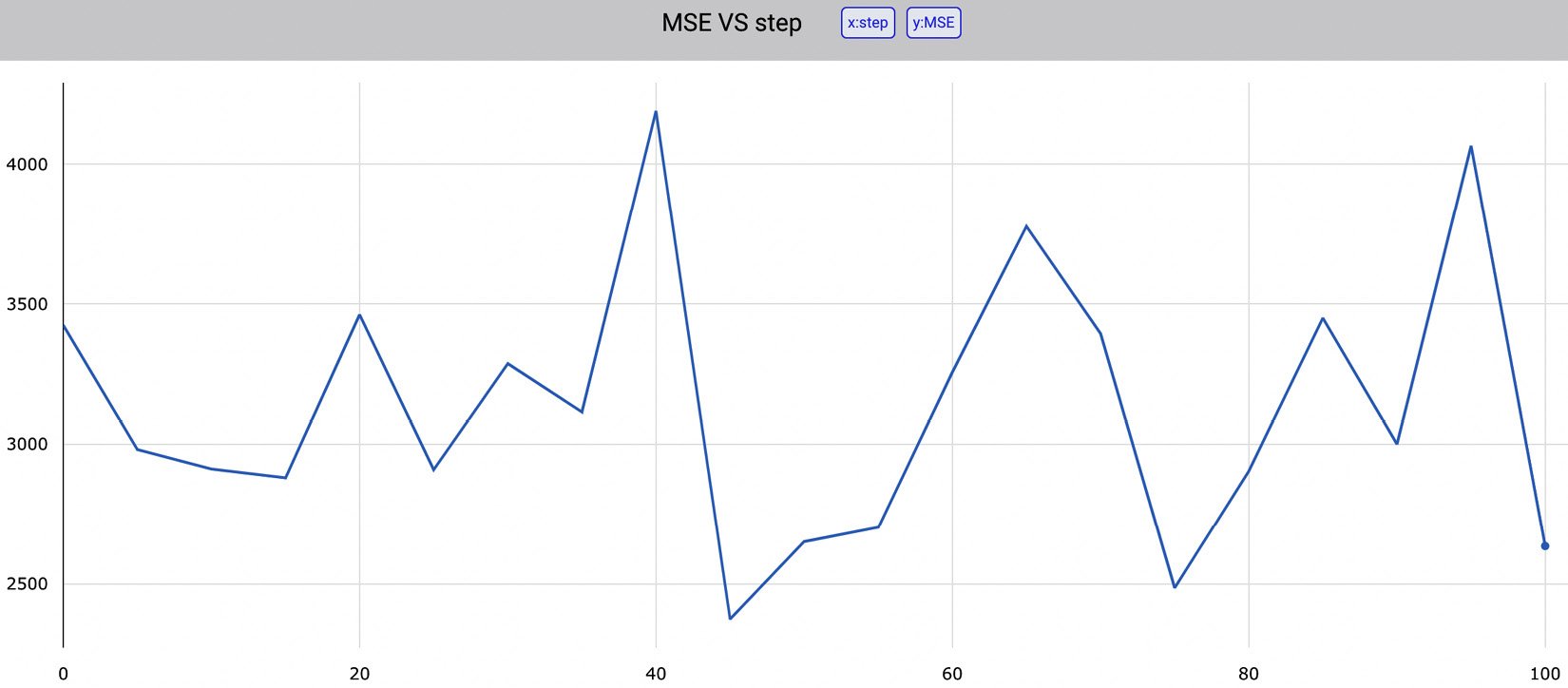
Under the Charts section, Comet shows all the graphs produced by our code. In our case, there is only one graph referring to MSE, as shown in the following figure:

Figure 1.18 – The value of MSE for different seeds provided as input to train_test_split()
The figure shows how the value of MSE depends on the seed value provided as input to the train_test_split() function. The produced graph is interactive, so we can view every single value in the trend line. We can download all the graphs as .jpeg or .svg files. In addition, we can download as a .json file of the data that has generated the graph. The following piece of code shows the generated JSON:
[{"x": [0,5,10,15,20,25,30,35,40,45,50,55,60,65,70,75,80,85,90,95],
"y":[3424.3166882137334,2981.5854714667616,2911.8279516891607,2880.7211416534115,3461.6357411723743,2909.472185919797,3287.490246176432,3115.203798301772,4189.681600195272,2374.3310824431856,2650.9384531241985,2702.2483323059314,3257.2142019316807,3776.092087838954,3393.8576719100192,2485.7719017765257,2904.0610865479025,3449.620077951196,3000.56755060663,4065.6795384526854],
"type":"scattergl",
"name":"MSE"}]
The previous code shows that there are two variables, x and y, and that the type of graph is scattergl.
Under the Metrics section, Comet shows a table with all the logged metrics, as shown in the following figure:

Figure 1.19 – The Metrics section in Comet
For each metric, Comet shows the last, minimum, and maximum values, as well as the step that determined those values.
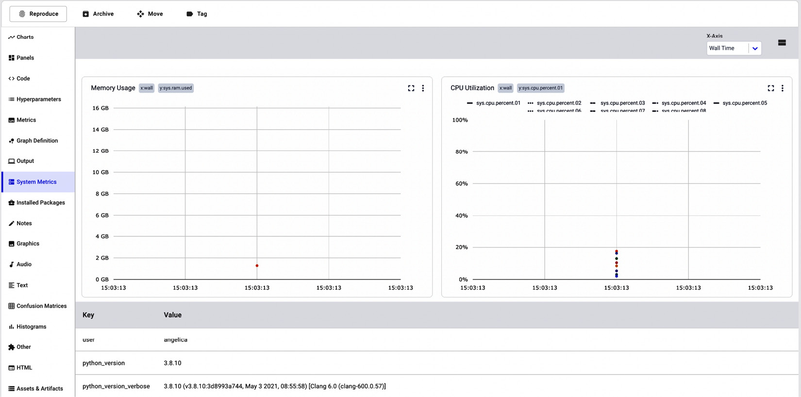
Finally, under the System Metrics section, Comet shows some metrics about the system conditions, including memory usage and CPU utilization, as well as the Python version and the type of operating system, as shown in the following figure:

Figure 1.20 – System Metrics in Comet
The System Metrics section shows two graphs, one for memory usage (on the left in the figure) and the other for the CPU utilization (on the right in the figure). Under the graph, the System Metrics section also shows a table with other useful information regarding the machine that generated the experiment.


