Comparing position-sizing algorithms

Let's take an example to further illustrate the principle. Let's use the exact same signals and starting capital. Then, let's use various position-sizing algorithms. Let's compute the equity curve for each position-sizing algorithm. The objective is to see how much position sizing impacts returns.

For demonstration purposes, we will recycle our go-to Softbank in absolute with Turtle for dummies, along with our regime_breakout() function from Chapter 5, Regime Definition. Once again, please do not do this at home, as it is too simplistic to be deployed in a professional investment product:

def regime_breakout(df,_h,_l,window):
    hl =  np.where(df[_h] == df[_h].rolling(window).max(),1,
                                np.where(df[_l] == df[_l].rolling(window).min(), -1,np.nan))
    roll_hl = pd.Series(index= df.index, data= hl).fillna(method= 'ffill')
    return roll_hl
 
def turtle_trader(df, _h, _l, slow, fast):
#### removed for brevity: check GitHub repo for full code ####
    return turtle
# CHAPTER 8
 
ticker = '9984.T' # Softbank
start = '2017-12-31'
end = None
df =  round(yf.download(tickers= ticker,start= start, end = end, 
                        interval = "1d",group_by = 'column',auto_adjust = True, 
                              prepost = True, treads = True, proxy = None),0)
 
ccy_ticker = 'USDJPY=X'
ccy_name = 'JPY'
ccy_df = np.nan
 
df[ccy_name] =  round(yf.download(tickers= ccy_ticker,start= start, end = end, 
                        interval = "1d",group_by = 'column',auto_adjust = True, 
                              prepost = True, treads = True, proxy = None)['Close'],2)
df[ccy_name] = df[ccy_name].fillna(method='ffill')
slow = 50
fast = 20 
df['tt'] = turtle_trader(df, _h= 'High', _l= 'Low', slow= slow,fast= fast)
df['tt_chg1D'] = df['Close'].diff() * df['tt'].shift()
df['tt_chg1D_fx'] = df['Close'].diff() * df['tt'].shift() / df[ccy_name]
 
df['tt_log_returns'] = np.log(df['Close'] / df['Close'].shift()) * df['tt'].shift()
df['tt_cumul_returns'] = df['tt_log_returns'].cumsum().apply(np.exp) - 1 
 
df['stop_loss'] = np.where(df['tt'] == 1, df['Low'].rolling(fast).min(),
                    np.where(df['tt'] == -1, df['High'].rolling(fast).max(),np.nan))# / df[ccy_name]
df['tt_PL_cum'] = df['tt_chg1D'].cumsum()
df['tt_PL_cum_fx'] = df['tt_chg1D_fx'].cumsum()
 
df[['Close','stop_loss','tt','tt_cumul_returns']].plot(secondary_y=['tt','tt_cumul_returns'],
                                  figsize=(20,10),style= ['k','r--','b:','b'],
                       title= str(ticker)+' Close Price, Turtle L/S entries')
 
df[['tt_chg1D','tt_chg1D_fx']].plot(secondary_y=['tt_chg1D_fx'],
                                  figsize=(20,10),style= ['b','c'],
                                 title= str(ticker) +' Daily P&L Local & USD')
 
df[['tt_PL_cum','tt_PL_cum_fx']].plot(secondary_y=['tt_PL_cum_fx'],
                                  figsize=(20,10),style= ['b','c'],
                                 title= str(ticker) +' Cumulative P&L Local & USD')       

This is our go-to example. Typically, today we have a signal at the close of the day. Tomorrow we will enter or exit. Entries and exits lag signals by one day using the shift method. We calculate cumulative returns (tt_cumul_returns) and daily profit and loss (tt_chg1D). This gives us the following graphs:

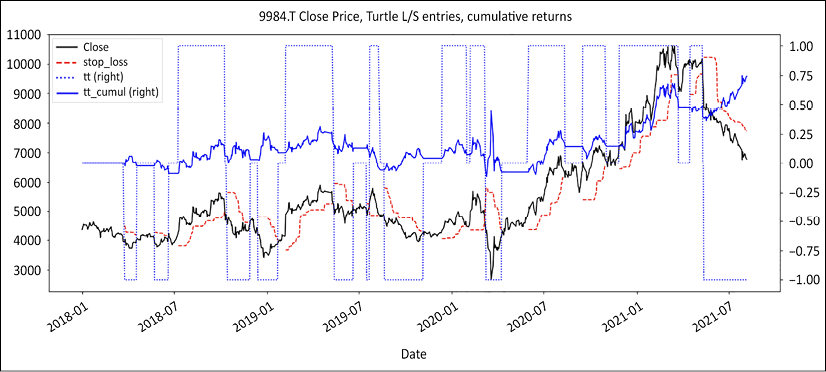
Figure 8.7: Softbank closing price, long/short positions, using Turtle for dummies on absolute series

The above chart sums up the strategy. With the black solid line, we have the closing price, closely followed by the red dashed stop loss line. We then have the +/-1 dotted line symbolizing long/short positions. Finally, the solid blue line represents cumulative returns.

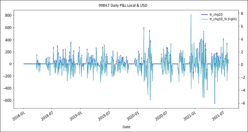
Figure 8.8: Strategy daily profit and loss in local currency and USD

The above chart represents the daily profit and loss in both local currency and adjusted to USD. The flat line shows when there is no active position.

Figure 8.9: Strategy cumulative profit and loss in local currency and USD

The above chart represents the cumulative profit and loss in local currency and USD. We use the same strategy on the same instrument with no additional features such as benchmark or liquidity adjustment. Everything is rigorously identical. The only difference is the position-sizing algorithm.

Let's define a few standard position-sizing algorithms. Equal weight is not defined below as it is a numerical constant, of 3% of equity. Rather than complicate things with more exotic position-sizing algorithms, let's keep it simple. We will use two of the most popular position-sizing algorithms: equal weight and equity at risk. We will then compare them with this concave and convex equity at risk. The latter two are new to the game. First, the source code for equity at risk is as follows:

def eqty_risk_shares(px,sl,eqty,risk,fx,lot):
    r = sl - px
    if fx > 0:
        budget = eqty * risk * fx
    else:
        budget = eqty * risk
    shares = round(budget // (r *lot) * lot,0)
#     print(r,budget,round(budget/r,0))
    return shares
 
px = 2000
sl = 2222
 
eqty = 100000
risk = -0.005
fx = 110
lot = 100
 
eqty_risk_shares(px,sl,eqty,risk,fx,lot)

This produces the following output:

-300.0

The above function returns a number of shares using price (px), stop loss denominated in local currency (sl), equity (eqty), risk, fx in fund currency, the currency in which the fund operates, and lot size. In the above example, this would return -300 shares.

Next, we run the simulation with 4 position-sizing algorithms: equal weight, constant, concave, and convex equity at risk:

starting_capital = 1000000
lot = 100
mn = -0.0025
mx = -0.0075
avg = (mn + mx) / 2
tolerance= -0.1
equal_weight = 0.05
shs_fxd = shs_ccv = shs_cvx = shs_eql = 0
df.loc[df.index[0],'constant'] = df.loc[df.index[0],'concave'] = starting_capital
df.loc[df.index[0],'convex'] = df.loc[df.index[0],'equal_weight'] = starting_capital
 
for i in range(1,len(df)):
    df['equal_weight'].iat[i] = df['equal_weight'].iat[i-1] + df['tt_chg1D_fx'][i] * shs_eql
    df['constant'].iat[i] = df['constant'].iat[i-1] + df['tt_chg1D_fx'][i] * shs_fxd
    df['concave'].iat[i] = df['concave'].iat[i-1] + df['tt_chg1D_fx'][i] * shs_ccv
    df['convex'].iat[i] = df['convex'].iat[i-1] + df['tt_chg1D_fx'][i] * shs_cvx
    
    ccv = risk_appetite(eqty= df['concave'][:i], tolerance=tolerance, 
                        mn= mn, mx=mx, span=5, shape=-1)
    cvx = risk_appetite(eqty= df['convex'][:i], tolerance=tolerance, 
                        mn= mn, mx=mx, span=5, shape=1)
 
    if (df['tt'][i-1] ==0) & (df['tt'][i] !=0):
        px = df['Close'][i]
        sl = df['stop_loss'][i]
        fx  = df[ccy_name][i]
        shs_eql = (df['equal_weight'].iat[i]  * equal_weight  *fx//(px * lot)) * lot
        if px != sl:
            shs_fxd = eqty_risk_shares(px,sl,eqty= df['constant'].iat[i],
                                        risk= avg,fx=fx,lot=100)
            shs_ccv = eqty_risk_shares(px,sl,eqty= df['concave'].iat[i],
                                            risk= ccv[-1],fx=fx,lot=100)
            shs_cvx = eqty_risk_shares(px,sl,eqty= df['convex'].iat[i],
                                            risk= cvx[-1],fx=fx,lot=100)
 
df[['constant','concave','convex','equal_weight', 'tt_PL_cum_fx']].plot(figsize = (20,10), grid=True,
    style=['y.-','m--','g-.','b:', 'b'],secondary_y='tt_PL_cum_fx',
title= 'cumulative P&L, concave, convex, constant equity at risk, equal weight ')

The code takes the following steps:

1. First we instantiate parameters such as the starting capital, currency, minimum and maximum risk, drawdown tolerance and equal weight.
2. We initialize the number of shares for each posSizer. We initialize the starting capital for each posSizer as well.
3. We loop through every bar to recalculate every equity curve by adding the previous value to the current number of shares times daily profit.
4. We recalculate the concave and convex risk oscillator at each bar.
5. If there is an entry signal, we calculate the number of shares for each posSizer. The // operator is modulo. It returns the rounded integer of the division. This is a neat trick to quickly calculate round lots. Note that the only difference between concave and convex is the sign: –1 or +1.

We then print the equity curves and voila. The dashed line at the top is concave. Below, the dash-dotted line is convex, followed by constant. The secondary vertical axis represents the cumulative profit and loss before weight adjustment:

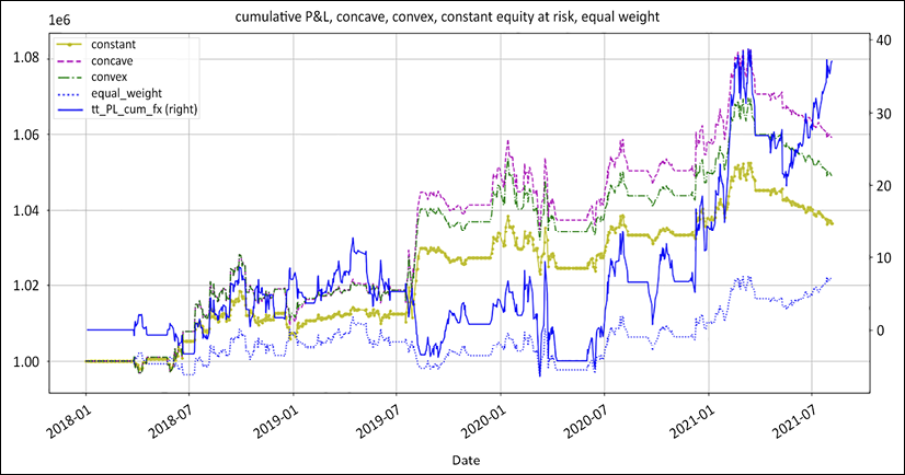
Figure 8.10: Equity curves using various position-sizing algorithms

Let's briefly recap here. We use the same strategy, in which cumulative returns adjusted for currency are represented by the solid blue line above. The only difference is money management. Trailing far away in a distant galaxy is the industry's standard equal weight. In this case, we use 5% of equity, a position size that seasoned institutional managers would call a "high-conviction" bet. A good second last is constant equity at risk. It is either first or fifth gear. Concave equity at risk surprisingly came first. Convex tends to perform better in choppy markets because of its responsiveness, while concave does well in trending markets.

The tectonic takeaway is that money is made in the money management module. How smart you bet determines how much you make. The best return on investment does not come from visiting one more company, making one more phone call, reading one more analyst report, or examining one more chart analysis. The best return on investment comes from polishing the money management module.