Search icon CANCEL
Subscription
0
Cart icon
Your Cart (0 item)
Close icon
You have no products in your basket yet
Arrow left icon
Explore Products
Best Sellers
New Releases
Books
Videos
Audiobooks
Learning Hub
Free Learning
Arrow right icon
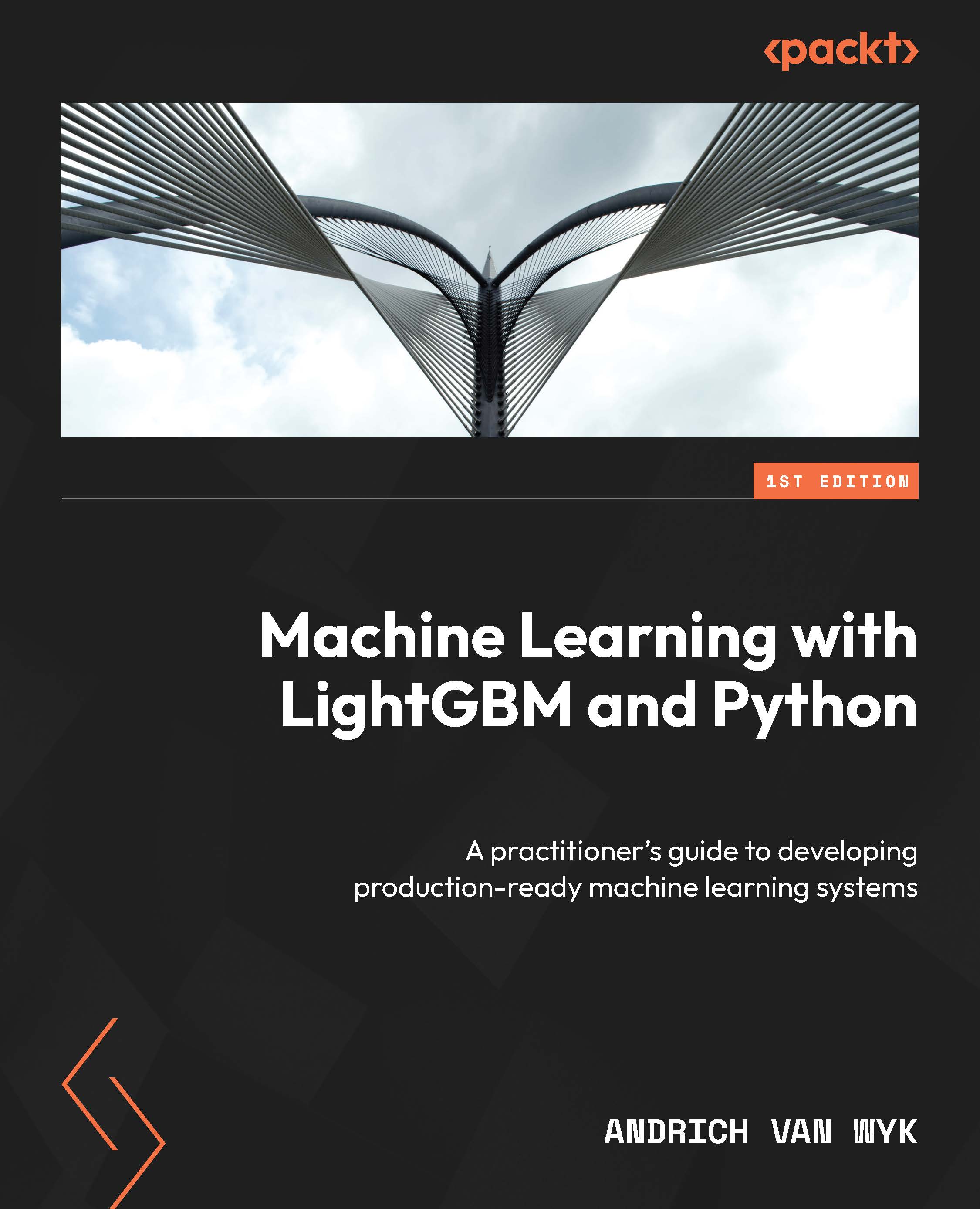
Machine Learning with LightGBM and Python

Machine Learning with LightGBM and Python: A practitioner's guide to developing production-ready machine learning systems

eBook
€8.99 €29.99
Paperback
€37.99
Subscription
Free Trial
Renews at €18.99p/m

What do you get with eBook?

Product feature icon Instant access to your Digital eBook purchase
Product feature icon Download this book in EPUB and PDF formats
Product feature icon Access this title in our online reader with advanced features
Product feature icon DRM FREE - Read whenever, wherever and however you want
OR
Modal Close icon
Payment Processing...
tick Completed

Billing Address

Table of content icon View table of contents Preview book icon Preview Book

Machine Learning with LightGBM and Python

Introducing Machine Learning

Our journey starts with an introduction to machine learning and the fundamental concepts we’ll use throughout this book.

We’ll start by providing an overview of machine learning from a software engineering perspective. Then, we’ll introduce the core concepts that are used in the field of machine learning and data science: models, datasets, learning paradigms, and other details. This introduction will include a practical example that clearly illustrates the machine learning terms discussed.

We will also introduce decision trees, a crucially important machine learning algorithm that is our first step to understanding LightGBM.

After completing this chapter, you will have established a solid foundation in machine learning and the practical application of machine learning techniques.

The following main topics will be covered in this chapter:

  • What is machine learning?
  • Introducing models, datasets, and supervised learning
  • Decision tree learning

Technical requirements

This chapter includes examples of simple machine learning algorithms and introduces working with scikit-learn. You must install a Python environment with scikit-learn, NumPy, pandas, and Jupyter Notebook. The code for this chapter is available at https://github.com/PacktPublishing/Practical-Machine-Learning-with-LightGBM-and-Python/tree/main/chapter-1.

What is machine learning?

Machine learning is a part of the broader artificial intelligence field that involves methods and techniques that allow computers to “learn” specific tasks without explicit programming.

Machine learning is just another way to write programs, albeit automatically, from data. Abstractly, a program is a set of instructions that transforms inputs into specific outputs. A programmer’s job is to understand all the relevant inputs to a computer program and develop a set of instructions to produce the correct outputs.

However, what if the inputs are beyond the programmer’s understanding?

For example, let’s consider creating a program to forecast the total sales of a large retail store. The inputs to the program would be various factors that could affect sales. We could imagine factors such as historical sales figures, upcoming public holidays, stock availability, any special deals the store might be running, and even factors such as the weather forecast or proximity to other stores.

In our store example, the traditional approach would be to break down the inputs into manageable, understandable (by a programmer) pieces, perhaps consult an expert in store sales forecasting, and then devise handcrafted rules and instructions to attempt to forecast future sales.

While this approach is certainly possible, it is also brittle (in the sense that the program might have to undergo extensive changes regarding the input factors) and wholly based on the programmer’s (or domain expert’s) understanding of the problem. With potentially thousands of factors and billions of examples, this problem becomes untenable.

Machine learning offers us an alternative to this approach. Instead of creating rules and instructions, we repeatedly show the computer examples of the tasks we need to accomplish and then get it to figure out how to solve them automatically.

However, where we previously had a set of instructions, we now have a trained model instead of a programmed one.

The key realization here, especially if you are coming from a software background, is that our machine learning program still functions like a regular program: it accepts input, has a way to process it, and produces output. Like all other software programs, machine learning software must be tested for correctness, integrated into other systems, deployed, monitored, and optimized. Collectively, this forms the field of machine learning engineering. We’ll cover all these aspects and more in later chapters.

Machine learning paradigms

Broadly speaking, machine learning has three main paradigms: supervised, unsupervised, and reinforcement learning.

With supervised learning, the model is trained on labeled data: each instance in the dataset has its associated correct output, or label, for the input example. The model is expected to learn to predict the label for unseen input examples.

With unsupervised learning, the examples in the dataset are unlabeled; in this case, the model is expected to discover patterns and relationships in the data. Examples of unsupervised approaches are clustering algorithms, anomaly detection, and dimensionality reduction algorithms.

Finally, reinforcement learning entails a model, usually called an agent, interacting with a particular environment and learning by receiving penalties or rewards for specific actions. The goal is for the agent to perform actions that maximize its reward. Reinforcement learning is widely used in robotics, control systems, or training computers to play games.

LightGBM and most other algorithms discussed later in this book are examples of supervised learning techniques and are the focus of this book.

The following section dives deeper into the machine learning terminology we’ll use throughout this book and the details of the machine learning process.

Introducing models, datasets, and supervised learning

In the previous section, we introduced a model as a construct to replace a set of instructions that typically comprise a program to perform a specific task. This section covers models and other core machine learning concepts in more detail.

Models

More formally, a model is a mathematical or algorithmic representation of a specific process that performs a particular task. A machine learning model learns a particular task by being trained on a dataset using a training algorithm.

Note

An alternative term for training is fit. Historically, fit stems from the statistical field. A model is said to “fit the data” when trained. We’ll use both terms interchangeably throughout this book.

Many distinct types of models exist, all of which use different mathematical, statistical, or algorithmic techniques to model the training data. Examples of machine learning algorithms include linear regression, logistic regression, decision trees, support vector machines, and neural networks.

A distinction is made between the model type and a trained instance of that model: the majority of machine learning models can be trained to perform various tasks. For example, decision trees (a model type) can be trained to forecast sales, recognize heart disease, and predict football match results. However, each of these tasks requires a different instance of a decision tree that has been trained on a distinct dataset.

What a specific model does depends on the model’s parameters. Parameters are also sometimes called weights, which are technically particular types of model parameters.

A training algorithm is an algorithm for finding the most appropriate model parameters for a specific task.

We determine the quality of fit, or how well the model performs, using an objective function. This is a mathematical function that measures the difference between the predicted output and the actual output for a given input. The objective function quantifies the performance of a model. We may seek to minimize or maximize the objective function depending on the problem we are solving. The objective is often measured as an error we aim to minimize during training.

We can summarize the model training process as follows: a training algorithm uses data from a dataset to optimize a model’s parameters for a particular task, as measured through an objective function.

Hyperparameters

While a model is composed of parameters, the training algorithm has parameters of its own called hyperparameters. A hyperparameter is a controllable value that influences the training process or algorithm. For example, consider finding the minimum of a parabola function: we could start by guessing a value and then take small steps in the direction that minimizes the function output. The step size would have to be chosen well: if our steps are too small, it will take a prohibitively long time to find the minimum. If the step size is too large, we may overshoot and miss the minimum and then continue oscillating (jumping back and forth) around the minimum:

Figure 1.1 – Effect of using a step size that is too large (left) and too small (right)

Figure 1.1 – Effect of using a step size that is too large (left) and too small (right)

In this example, the step size would be a hyperparameter of our minimization algorithm. The effect of the step size is illustrated in Figure 1.1.

Datasets

As explained previously, the machine learning model is trained using a dataset. Data is at the heart of the machine learning process, and data preparation is often the part of the process that takes up the most time.

Throughout this book, we’ll work with tabular datasets. Tabular datasets are very common in the real world and consist of rows and columns. Rows are often called samples, examples, or observations, and columns are usually called features, variables, or attributes.

Importantly, there is no restriction on the data type in a column. Features may be strings, numbers, Booleans, geospatial coordinates, or encoded formats such as audio, images, or video.

Datasets are also rarely perfectly defined. Data may be incomplete, noisy, incorrect, inconsistent, and contain various formats.

Therefore, data preparation and cleaning are essential parts of the machine learning process.

Data preparation concerns processing the data to make it suitable for machine learning and typically consists of the following steps:

  1. Gathering and validation: Some datasets are initially too small or represent the problem poorly (the data is not representative of the actual data population it’s been sampled from). In these cases, the practitioner must collect more data, and validation must be done to ensure the data represents the problem.
  2. Checking for systemic errors and bias: It is vital to check for and correct any systemic errors in the collection and validation process that may lead to bias in the dataset. In our sales example, a systemic collection error may be that data was only gathered from urban stores and excluded rural ones. A model trained on only urban store data will be biased in forecasting store sales, and we may expect poor performance when the model is used to predict sales for rural stores.
  3. Cleaning the data: Any format or value range inconsistencies must be addressed. Any missing values also need to be handled in a way that does not introduce bias.
  4. Feature engineering: Certain features may need to be transformed to ensure the machine learning model can learn from them, such as numerically encoding a sentence of words. Additionally, new features may need to be prepared from existing features to help the model detect patterns.
  5. Normalizing and standardizing: The relative ranges of features must be normalized and standardized. Normalizing and standardizing ensure that no one feature has an outsized effect on the overall prediction.
  6. Balancing the dataset: In cases where the dataset is imbalanced – that is, it contains many more examples of one class or prediction than another – the dataset needs to be balanced. Balancing is typically done by oversampling the minority examples to balance the dataset.

In Chapter 6, Solving Real-World Data Science Problems with LightGBM, we’ll go through the entire data preparation process to show how the preceding steps are applied practically.

Note

A good adage to remember is “garbage in, garbage out”. A model learns from any data given to it, including any flaws or biases contained in the data. When we train the model on garbage data, it results in a garbage model.

One final concept to understand regarding datasets is the training, validation, and test datasets. We split our datasets into these three subsets after the data preparation step is done:

  • The training set is the most significant subset and typically consists of 60% to 80% of the data. This data is used to train the model.
  • The validation set is separate from the training data and is used throughout the training process to evaluate the model. Having independent validation data ensures that the model is evaluated on data it has not seen before, also known as its generalization ability. Hyperparameter tuning, a process covered in detail in Chapter 5, LightGBM Parameter Optimization with Optuna, also uses the validation set.
  • Finally, the test set is an optional hold-out set, similar to the validation set. It is used at the end of the process to evaluate the model’s performance on data that was not part of the training or tuning process.

Another use of the validation set is to monitor whether the model is overfitting the data. Let’s discuss overfitting in more detail.

Overfitting and generalization

To understand overfitting, we must first define what we mean by model generalization. As stated previously, generalization is the model’s ability to accurately predict data it has not seen before. Compared to training accuracy, generalization accuracy is more significant as an estimate of model performance as this indicates how our model will perform in production. Generalization comes in two forms, interpolation and extrapolation:

  • Interpolation refers to the model’s ability to predict a value between two known data points – stated another way, to generalize within the training data range. For example, let’s say we train our model with monthly data from January to July. When interpolating, we would ask the model to make a prediction on a particular day in April, a date within our training range.
  • Extrapolation, as you might infer, is the model’s ability to predict values outside of the range defined by our training data. A typical example of extrapolation is forecasting – that is, predicting the future. In our previous example, if we ask the model to make a prediction in December, we expect it to extrapolate from the training data.

Of the two types of generalization, extrapolation is much more challenging and may require a specific type of model to achieve. However, in both cases, a model can overfit the data, losing its ability to interpolate or extrapolate accurately.

Overfitting is a phenomenon where the model fits the training data too closely and loses its ability to generalize to unseen data. Instead of learning the underlying pattern in the data, the model has memorized the training data. More technically, the model fits the noise contained in the training data. The term noise stems from the concept of data containing signal and noise. Signal refers to the underlying pattern or information captured in the data we are trying to predict. In contrast, noise refers to random or irrelevant variations of data points that mask the signal.

For example, consider a dataset where we try to predict the rainfall for specific locations. The signal in the data would be the general trend of rainfall: rainfall increases in the winter or summer, or vice versa for other locations. The noise would be the slight variations in rainfall measurement for each month and location in our dataset.

The following graph illustrates the phenomenon of overfitting:

Figure 1.2 – Graph showing overfitting. The model has overfitted and predicted the training data perfectly but has lost the ability to generalize to the actual signal

Figure 1.2 – Graph showing overfitting. The model has overfitted and predicted the training data perfectly but has lost the ability to generalize to the actual signal

The preceding figure shows the difference between signal and noise: each data point was sampled from the actual signal. The data follows the general pattern of the signal, with slight, random variations. We can see how the model has overfitted the data: the model has fit the training data perfectly but at the cost of generalization. We can also see that if we use the model to interpolate by predicting a value for 4, we get a result much higher than the actual signal (6.72 versus 6.2). Also shown is the model’s failure to extrapolate: the prediction for 12 is much lower than a forecast of the signal (7.98 versus 8.6).

In reality, all real-world datasets contain noise. As data scientists, we aim to prepare the data to remove as much noise as possible, making the signal easier to detect. Data cleaning, normalization, feature selection, feature engineering, and regularization are techniques for removing noise from the data.

Since all real-world data contains noise, overfitting is impossible to eliminate. The following conditions may lead to overfitting:

  • An overly complex model: A model that is too complex for the amount of data we have utilizes additional complexity to memorize the noise in the data, leading to overfitting
  • Insufficient data: If we don’t have enough training data for the model we use, it’s similar to an overly complex model, which overfits the data
  • Too many features: A dataset with too many features likely contains irrelevant (noisy) features that reduce the model’s generalization
  • Overtraining: Training the model for too long allows it to memorize the noise in the dataset

As the validation set is a part of the training data that remains unseen by the model, we use the validation set to monitor for overfitting. We can recognize the point of overfitting by looking at the training and generalization errors over time. At the point of overfitting, the validation error increases. In contrast, the training error continues to improve: the model is fitting noise in the training data and losing its ability to generalize.

Techniques that prevent overfitting usually aim to address the conditions that lead to overfitting we discussed previously. Here are some strategies to avoid overfitting:

  • Early stopping: We can stop training when we see the validation error beginning to increase.
  • Simplifying the model: A less complex model with fewer parameters would be incapable of learning the noise in the training data, thereby generalizing better.
  • Get more data: Either collecting more data or augmenting data is an effective method for preventing overfitting by giving the model a better chance to learn the signal in the data instead of the noise in a smaller dataset.
  • Feature selection and dimensionality reduction: As some features might be irrelevant to the problem being solved, we can discard features we think are redundant or use techniques such as Principal Component Analysis to reduce the dimensionality (features).
  • Adding regularization: Smaller parameter values typically lead to better generalization, depending on the model (a neural network is an example of such a model). Regularization adds a penalty term to the objective function to discourage large parameter values. By driving the parameters to smaller (or zero) values, they contribute less to the prediction, effectively simplifying the model.
  • Ensemble methods: Combining the prediction from multiple, weaker models can lead to better generalization while also improving performance.

It’s important to note that overfitting and the techniques to prevent overfitting are specific to our model. Our goal should always be to minimize overfitting to ensure generalization to unseen data. Some strategies, such as regularization, might not work for specific models, while others might be more effective. There are also more bespoke strategies for models, an example of which we’ll see when we discuss overfitting in decision trees.

Supervised learning

The store sales example is an instance of supervised learning – we have a dataset consisting of features and are training the model to predict a target.

Supervised learning problems can be divided into two main types of problem categories: classification problems and regression problems.

Classification and regression

With a classification problem, the label that needs to be predicted by the model is categorical or defines a class. Some examples of classes are spam or not spam, cat or dog, and diabetic or not diabetic. These are examples of binary classifications: there are only two classes.

Multi-class classification is also possible; for example, email may be classified as Important, Promotional, Clutter, or Spam; images of clouds could be classified as Cirro, Cumulo, Strato, or Nimbo.

With regression problems, the goal is to predict a continuous, numerical value. Examples include predicting revenue, sales, temperature, house prices, and crowd size.

A big part of the art of machine learning is correctly defining or transcribing a problem as a classification or regression problem (or perhaps unsupervised or reinforcement). Later chapters will cover multiple end-to-end case studies of both types of problems.

Model performance metrics

Let’s briefly discuss how we measure our model’s performance. Model performance refers to the ability of a machine learning model to make accurate predictions or generate meaningful outputs based on the given inputs. An evaluation metric quantifies how well a model generalizes to new, unseen data. High model performance indicates that the model has learned the underlying patterns in the data effectively and can make accurate predictions on data it has not seen before. We can measure the model’s performance relative to the known targets when working with supervised learning problems (either classification or regression problems).

Importantly, how we measure the model’s performance on classification tasks and regression tasks differs. scikit-learn has many built-in metrics functions ready for use with either a classification or regression problem (https://scikit-learn.org/stable/modules/model_evaluation.html). Let’s review the most common of these.

Classification metrics can be defined in terms of positive and negative predictions made by the model. The following definitions can be used to calculate classification metrics:

  • True positive (TP): A positive instance is correctly classified as positive
  • True negative (TN): A negative instance is correctly classified as negative
  • False positive (FP): A negative instance is incorrectly classified as positive
  • False negative (FN): A positive instance is incorrectly classified as negative

Given these definitions, the most common classification metrics are as follows:

  • Accuracy: Accuracy is the most straightforward classification metric. Accuracy is the number of correct predictions divided by the total number of predictions. However, accuracy is susceptible to an imbalance in the data. For example, suppose we have an email dataset with 8 examples of spam and 2 examples of non-spam, and our model predicts only spam. In that case, the model has an accuracy of 80%, even though it never correctly classified non-spam emails. Mathematically, we can define accuracy as follows:

    Accuracy =  TP + TN ______________  TP + FP + TN + FN 

  • Precision: The precision score is one way of getting a more nuanced understanding of the classification performance. Precision is the ratio between the true positive prediction (correctly predicted) and all positive predictions (true positive and false positive). In other words, the precision score indicates how precise the model is in predicting positives. In our spam emails example, a model predicting only spam is not very precise (as it classifies all non-spam emails as spam) and has a lower precision score. The following formula can be used to calculate precision:

    Precision =  TP _ TP + FP 

  • Recall: The recall score is the counterpoint to the precision score. The recall score measures how effectively the model finds (or recalls) all true positive cases. The recall is calculated as the ratio between true positive predictions and all positive instances (true positive and false negative). In our spam example, a model predicting only spam has perfect recall (it can find all the spam). We can calculate recall like so:

    Recall =  TP _ TP + FN 

  • F1 score: Finally, we have the F1 score. The F1 score is calculated as the harmonic mean between precision and recall. The F1 score balances precision and recall, giving us a singular value that summarizes the classifier’s performance. The following formula can be used to calculate the F1 score:

    F 1 =  2 × Precision × Recall  _______________  Precision + Recall  =  2 × TP _____________  2 × TP + FP + FN 

The preceding classification metrics are the most common, but there are many more. Even though the F1 score is commonly used in classification problems (as it summarizes precision and recall), choosing the best metric is specific to the problem you are solving. Often, it might be the case that a specific metric is required, but other times, you must choose based on experience and your understanding of the data. We will look at examples of different metrics later in this book.

The following are common regression metrics:

  • Mean squared error (MSE): The MSE is calculated as the average of the squared differences between predicted and actual values. The MSE is commonly used because of one crucial mathematical property: the MSE is differentiable and is therefore appropriate for use with gradient-based learning methods. However, since the difference is squared, the MSE penalizes large errors more heavily than small errors, which may or may not be appropriate to the problem being solved.
  • Mean absolute error (MAE): Instead of squaring the differences, the MAE is calculated as the average of the absolute differences between predicted and actual values. By avoiding the square of errors, the MAE is more robust against the magnitude of errors and less sensitive to outliers than the MSE. However, the MAE is not differentiable and, therefore, can’t be used with gradient-based learning methods.

As with the classification metrics, choosing the most appropriate regression metric is specific to the problem you are trying to solve.

Metrics versus objectives

We defined training a model as finding the most appropriate parameters to minimize an objective function. It’s important to note that the objective function and metrics used for a specific problem may differ. A good example is decision trees, where a measure of impurity (entropy) is used as the objective function when building a tree. However, we still calculate the metrics explained previously to determine the tree’s performance on the data.

With our understanding of basic metrics in place, we can conclude our introduction to machine learning concepts. Now, let’s review the terms and concepts we’ve discussed using an example.

A modeling example

Consider the following data of sales by month, in thousands:

Jan

Feb

Mar

Apr

May

Jun

4,140

4,850

7,340

6,890

8,270

10,060

Jul

Aug

Sept

Oct

Nov

Dec

8,110

11,670

10,450

11,540

13,400

14,420

Table 1.1 – Sample sales data, by month, in thousands

This problem is straightforward: there is only one feature, the month, and the target is the number of sales. Therefore, this is an example of a supervised regression problem.

Note

You might have noticed that this is an example of a time series problem: time is the primary variable. Time series can also be predicted using more advanced time series-specific algorithms such as ANOVA, but we’ll use a simple algorithm for illustration purposes in this section.

We can plot our data as a graph of sales per month to understand it better:

Figure 1.3 – Graph showing store sales by month

Figure 1.3 – Graph showing store sales by month

Here, we’re using a straight-line model, also known as simple linear regression, to model our sales data. The definition of a straight line is given by the following formula:

y = mx + c

Here, m is the line’s slope and c is the Y-intercept. In machine learning, the straight line is the model, and m and c are the model parameters.

To find the best parameters, we must measure how well our model fits the data for a particular set of parameters – that is, the error in our outputs. We will use the MAE as our metric:

MAE =   i=1 n  | ˆ y  y| _ n 

Here,  ˆ y  is the predicted output, y is the actual output, and n is the number of predictions. We calculate the MAE by making a prediction for each of our inputs and then calculating the MAE based on the formula.

Fitting the model

Now, let’s fit our linear model to our data. Our process for fitting the line is iterative, and we start this process by guessing values for m and c and then iterating from there. For example, let’s consider m = 0.1, c = 4:

Figure 1.4 – Graph showing the prediction of a linear model with m = 0.1 and c = 4

Figure 1.4 – Graph showing the prediction of a linear model with m = 0.1 and c = 4

With these parameters, we achieve an error of 4,610.

Our guess is far too low, but that’s okay; we can now update the parameters to attempt to improve the error. In reality, updating the model parameters is done algorithmically using a training algorithm such as gradient descent. We’ll discuss gradient descent in Chapter 2, Ensemble Learning – Bagging and Boosting.

In this example, we’ll use our understanding of straight lines and intuition to update the parameters for each iteration manually. Our line is too shallow, and the intercept is too low; therefore, we must increase both values. We can control the updates we make each iteration by choosing a step size. We must update the m and c values with each iteration by adding the step size. The results, for a step size of 0.1, is shown in Table 1.2.

Guess#

m

c

MAE

1

0.1

4

4.61

2

0.2

4.1

3.89

3

0.3

4.2

3.17

4

0.3

4.3

2.5

5

0.4

4.4

1.83

Table 1.2 – Step wise guessing of the slope (m) and y-intercept (c) for a straight line to fit our data. The quality of fit is measured using the MAE

In our example, the step size is a hyperparameter of our training process.

We end up with an error of 1.83, which means, on average, our predictions are wrong by less than 2,000.

Now, let’s see how we can solve this problem using scikit-learn.

Linear regression with scikit-learn

Instead of manually modeling, we can use scikit-learn to build a linear regression model. As this is our first example, we’ll walk through the code line by line and explain what’s happening.

To start with, we must import the Python tools we are going to use:

import numpy as np
import pandas as pd
from matplotlib import pyplot as plt
import seaborn as sns
from sklearn.linear_model import LinearRegression
from sklearn.metrics import mean_absolute_error

There are three sets of imports: we import numpy and pandas first. Importing NumPy and pandas is a widely used way to start all your data science notebooks. Also, note the short names np and pd, which are the standard conventions when working with numpy and pandas.

Next, we import a few standard plotting libraries we will use to plot some graphs: pyplot from matplotlib and seaborn. Matplotlib is a widely used plotting library that we access via the pyplot python interface. Seaborn is another visualization tool built on top of Matplotlib, which makes it easier to draw professional-looking graphs.

Finally, we get to our scikit-learn imports. In Python code, the scikit-learn library is called sklearn. From its linear_model package, we import LinearRegression. scikit-learn implements a wide variety of predefined metrics, and here, we will be using mean_absolute_error.

Now, we are ready to set up our data:

months = np.array([ 1,  2,  3,  4,  5,  6,  7,  8,  9, 10, 11, 12])
sales = np.array([4.14,  4.85,  7.34,  6.89,  8.27, 10.06,  8.11, 11.67, 10.45, 11.54, 13.4 , 14.42])
df = pd.DataFrame({"month": months, "sales": sales})

Here, we define a new numpy array for the months and the corresponding sales, and to make them easier to work with, we gather both arrays into a new pandas DataFrame.

With the data in place, we get to the interesting part of the code: modeling using scikit-learn. The code is straightforward:

model = LinearRegression()
model = model.fit(df[["month"]], df[["sales"]])

First, we create our model by constructing an instance of LinearRegression. We then fit our model using model.fit and passing in the month and sales data from our DataFrame. These two lines are all that’s required to fit a model, and as we’ll see in later chapters, even complicated models use the same recipe to instantiate and train a model.

We can now calculate our MAE by creating predictions for our data and passing the predictions and actual targets to the metric function:

predicted_sales = model.predict(df[["month"]])
mean_absolute_error(predicted_sales, df[["sales"]])

We get an error of 0.74, which is slightly lower than our guesswork. We can also examine the model’s coefficient and intercept (m and c from earlier):

print(f"Gradient: ${model.coef_}")
print(f"Intercept: ${model.intercept_}")

scikit-learn has fitted a model with a coefficient of 0.85 and an intercept of 3.68. We were in the right neighborhood with our guesses, but it might have taken us some time to get to the optimal values.

That concludes our introduction to scikit-learn and the basics of modeling and machine learning. In our toy example, we did not split our data into separate datasets, optimize our model’s hyperparameters, or apply any techniques to ensure our model does not overfit. In the next section, we’ll look at classification and regression examples, where we’ll apply these and other best practices.

Decision tree learning

This section introduces decision tree learning, a machine learning algorithm essential to understanding LightGBM. We’ll work through an example of how to build decision trees using scikit-learn. This section will also provide some mathematical definitions for building decision trees; understanding these definitions is not critical, but it will help us understand our discussion of the decision tree hyperparameters.

Decision trees are tree-based learners that function by asking successive questions about the data to determine the result. A path is followed down the tree, making decisions about the input using one or more features. The path terminates at a leaf node, which represents the predicted class or value. Decision trees can be used for classification or regression.

The following is an illustration of a decision tree fit on the Iris dataset:

Figure 1.5 – A decision tree modeling the Iris dataset

Figure 1.5 – A decision tree modeling the Iris dataset

The Iris dataset is a classification dataset where Iris flower sepal and petal dimensions are used to predict the type of Iris flower. Each non-leaf node uses one or more features to narrow down the samples in the dataset: the root node starts with all 150 samples and then splits them based on petal width, <= 0.8. We continue down the tree, with each node splitting the samples further until we reach a leaf node that contains the predicted class (versicolor, virginica, or setosa).

Compared to other models, decision trees have many advantages:

  • Features may be numeric or categorical: Samples can be split using either numerical features (by splitting a range) or categorical ones without us having to encode either.
  • Reduced need for data preparation: Decision splits are not sensitive to data ranges or size. Many other models (for example, neural networks) require data to be normalized to unit ranges.
  • Interpretability: As shown previously, it’s straightforward to interpret the predictions made by a tree. Interpretability is valuable in contexts where a prediction must be explained to decision-makers.

These are just some of the advantages of using tree-based models. However, we also need to be aware of some of the disadvantages associated with decision trees:

  • Overfitting: Decision trees are very prone to overfitting. Setting the correct hyperparameters is essential when fitting decision trees. Overfitting in decision trees will be discussed in detail later.
  • Poor extrapolation: Decision trees are poor at extrapolation since their predictions are not continuous and are effectively bounded by the training data.
  • Unbalanced data: When fitting a tree on unbalanced data, the high-frequency classes dominate the predictions. Data needs to be prepared to remove imbalances.

A more detailed discussion of the advantages and disadvantages of decision trees is available at https://scikit-learn.org/stable/modules/tree.html.

Entropy and information gain

First, we need a rudimentary understanding of entropy and information gain before we look at an algorithm for building (or fitting) a decision tree.

Entropy can be considered a way to measure the disorder or randomness of a system. Entropy measures how surprising the result of a specific input or event might be. Consider a well-shuffled deck of cards: drawing from the top of the deck could give us any of the cards in the deck (a surprising result each time); therefore, we can say that a shuffled deck of cards has high entropy. Drawing cards from the top of an ordered deck is unsurprising; we know which cards come next. Therefore, an ordered deck of cards has low entropy. Another way to interpret entropy is the impurity of the dataset: a low-entropy dataset (neatly ordered) has less impurity than a high-entropy dataset.

Information gain, in turn, is the amount of information gained when modifying or observing the underlying data. Information gain involves reducing entropy from before the observation. In our deck of cards example, we might take a shuffled deck of cards and split it into four smaller decks by suit (spades, hearts, diamonds, and clubs). If we draw from the smaller decks, the outcome is less of a surprise: we know that the next card is from the same suit. By splitting the deck by suit, we have reduced the entropy of the smaller decks. Splitting the deck of cards on a feature (the suit) is very similar to how the splits in a decision tree work; each division seeks to maximize the information gain – that is, they minimize the entropy after the split.

In decision trees, there are two common ways of measuring information gain or the loss of impurity:

  • The Gini index
  • Log loss or entropy

A detailed explanation of each is available at https://scikit-learn.org/stable/modules/tree.html#classification-criteria.

Building a decision tree using C4.5

C4.5 is an algorithm for building a decision tree from a dataset [1]. The algorithm is recursive and starts with the following base cases:

  1. If all the samples in a sub-dataset are of the same class, create a leaf node in the tree that chooses that class.
  2. If no information can be gained by splitting using any of the features (the dataset can’t be divided any further), create a leaf node that predicts the most frequent class contained in the sub-dataset.
  3. If a minimum threshold of samples is reached in a sub-dataset, create a leaf node that predicts the most frequent class contained in the sub-dataset.

Then, we can apply the algorithm:

  1. Check for any of the three base cases and stop splitting if any applies to the dataset.
  2. For each feature or attribute of the dataset, calculate the information gained by splitting the dataset on that feature.
  3. Create a decision node by splitting the dataset on the feature with the highest information gain.
  4. Split the dataset into two sub-datasets based on the decision node and recursively reply to the algorithm on each sub-dataset.

Once the tree has been built, pruning is applied. During pruning, decision nodes with a relatively lower information gain than other tree nodes are removed. Removing nodes avoids overfitting the training data and improves the tree’s generalization ability.

Classification and Regression Tree

You may have noticed that in the preceding explanations, we only used classes to split datasets using decision nodes; this is not by chance, as the canonical C4.5 algorithm only supports classification trees. Classification and Regression Tree (CART) extends C4.5 to support numerical target variables – that is, regression problems [2]. With CART, decision nodes can also split continuous numerical input variables to support regression, typically using a threshold (for example, x <= 0.3). When reaching a leaf node, the mean or median of the remaining numerical range is generally taken as the predicted value.

When building classification trees, only impurity is used to determine splits. However, with regression trees, impurity is combined with other criteria to calculate optimal splits:

  • The MSE (or MAE)
  • Half Poisson Deviance

A detailed mathematical explanation of each is available at https://scikit-learn.org/stable/modules/tree.html#regression-criteria.

scikit-learn uses an optimized version of CART to build decision trees.

Overfitting in decision trees

One of the most significant disadvantages of decision trees is that they are prone to overfitting. Without proper hyperparameter choices, C4.5 and other training algorithms create overly complex and deep trees that fit the training data almost exactly. Managing overfitting is a crucial part of building decision trees. Here are some strategies to avoid overfitting:

  • Pruning: As mentioned previously, we can remove branches that do not contribute much information gain; this reduces the tree’s complexity and improves generalization.
  • Maximum depth: Limiting the depth of the tree also avoids overly complex trees and avoids overfitting.
  • Maximum number of leaf nodes: Similar to restricting depth, limiting the number of leaf nodes avoids overly specific branches and improves generalization.
  • Minimum samples per leaf: Setting a minimum limit on the number of samples a leaf may contain (stopping splitting when the sub-dataset is of the minimum size) also avoids overly specific leaf nodes.
  • Ensemble methods: Ensemble learning is a technique that combines multiple models to improve the prediction over an individual model. Averaging the prediction of multiple models can also reduce overfitting.

These strategies can be applied by setting the appropriate hyperparameters. Now that we understand how to build decision trees and strategies for overfitting, let’s look at building decision trees in scikit-learn.

Building decision trees with scikit-learn

It is time to examine how we may use decision trees by training classification and regression trees using scikit-learn.

For these examples, we’ll use the toy datasets included in scikit-learn. These datasets are small compared to real-world data but are easy to work with, allowing us to focus on the decision trees.

Classifying breast cancer

We’ll use the Breast Cancer dataset (https://scikit-learn.org/stable/datasets/toy_dataset.html#breast-cancer-dataset) for our classification example. This dataset consists of features that have been calculated from the images of fine needle aspirated breast masses, and the task is to predict whether the mass is malignant or benign.

Using scikit-learn, we can solve this classification problem with five lines of code:

dataset = datasets.load_breast_cancer()
X_train, X_test, y_train, y_test = train_test_split(dataset.data, dataset.target, random_state=157)
model = DecisionTreeClassifier(random_state=157, max_depth=3, min_samples_split=2)
model = model.fit(X_train, y_train)
f1_score(y_test, model.predict(X_test))

First, we load the dataset using load_breast_cancer. Then, we split our dataset into training and test sets using train_test_split; by default, 25% of the data is used for the test set. Like before, we instantiate our DecisionTreeClassifier model and train it on the training set using model.fit. The two hyperparameters we pass through when instantiating the model are notable: max_depth and min_samples_split. Both parameters control overfitting and will be discussed in more detail in the next section. We also specify random_state for both the train-test split and the model. By fixing the random state, we ensure the outcome is repeatable (otherwise, a new random state is created by scikit-learn for every execution).

Finally, we measure the performance using f1_score. Our model achieves an F1 score of 0.94 and an accuracy of 93.7%. F1 scores are out of 1.0, so we may conclude that the model does very well. If we break down our predictions, the model missed the prediction on only 9 of the 143 samples in the test set: 7 false positives and 2 false negatives.

Predicting diabetes progression

To illustrate solving a regression problem with decision trees, we’ll use the Diabetes dataset (https://scikit-learn.org/stable/datasets/toy_dataset.html#diabetes-dataset). This dataset has 10 features (age, sex, body mass index, and others), and the model is tasked with predicting a quantitative measure of disease progression after 1 year.

We can use the following code to build and evaluate a regression model:

dataset = datasets.load_diabetes()
X_train, X_test, y_train, y_test = train_test_split(dataset.data, dataset.target, random_state=157)
model = DecisionTreeRegressor(random_state=157, max_depth=3, min_samples_split=2)
model = model.fit(X_train, y_train)
mean_absolute_error(y_test, model.predict(X_test))

Our model achieves an MAE of 45.28. The code is almost identical to our classification example: instead of a classifier, we use DecisionTreeRegressor as our model and calculate mean_absolute_error instead of the F1 score. The consistency in the API for solving various problems with different types of models in scikit-learn is by design and illustrates a fundamental truth in machine learning work: even though data, models, and metrics change, the overall process for building machine learning models remains the same. In the coming chapters, we’ll expand on this general methodology and leverage the process’ consistency when building machine learning pipelines.

Decision tree hyperparameters

We used some decision tree hyperparameters in the preceding classification and regression examples to control overfitting. This section will look at the most critical decision tree hyperparameters provided by scikit-learn:

  • max_depth: The maximum depth the tree is allowed to reach. Deeper trees allow more splits, resulting in more complex trees and overfitting.
  • min_samples_split: The minimum number of samples required to split a node. Nodes containing only a few samples overfit the data, whereas having a larger minimum improves generalization.
  • min_samples_leaf: The minimum number of samples allowed in leaf nodes. Like the minimum samples in a split, increasing the value leads to less complex trees, reducing overfitting.
  • max_leaf_nodes: The maximum number of lead nodes to allow. Fewer leaf nodes reduce the tree size and, therefore, the complexity, which may improve generalization.
  • max_features: The maximum features to consider when determining a split. Discarding some features reduces noise in the data, which improves overfitting. Features are chosen at random.
  • criterion: The impurity measure to use when determining a split, either gini or entropy/log_loss.

As you may have noticed, most decision tree hyperparameters involve controlling overfitting by controlling the complexity of the tree. These parameters provide multiple ways of doing so, and finding the best combination of parameters and their values is non-trivial. Finding the best hyperparameters is called hyperparameter tuning and will be covered extensively later in this book.

A complete list of the hyperparameters can be found at the following places:

Now, let’s summarize the key takeaways from this chapter.

Summary

In this chapter, we introduced machine learning as a method of creating software by learning to perform a task from a corpus of data instead of relying on programming the instructions by hand. We introduced the core concepts of machine learning with a focus on supervised learning and illustrated their applications through examples with scikit-learn.

We also introduced decision trees as a machine learning algorithm and discussed their strengths and weaknesses, as well as how to control overfitting using hyperparameters. We concluded this chapter with examples of how to solve classification and regression problems using decision trees in scikit-learn.

This chapter has given us a foundational understanding of machine learning, enabling us to dive deeper into the data science process and the LightGBM library.

The next chapter will focus on ensemble learning in decision trees, a technique where the predictions of multiple decision trees are combined to improve the overall performance. Boosting, particularly gradient boosting, will be covered in detail.

References

[1]

J. R. Quinlan, C4.5: Programs for machine learning, Elsevier, 2014.

[2]

R. J. Lewis, An introduction to classification and regression tree (CART) analysis, in Annual meeting of the Society For Academic Emergency Medicine in San Francisco, California, 2000.

Left arrow icon Right arrow icon
Download code icon Download Code

Key benefits

  • Get started with LightGBM, a powerful gradient-boosting library for building ML solutions
  • Apply data science processes to real-world problems through case studies
  • Elevate your software by building machine learning solutions on scalable platforms
  • Purchase of the print or Kindle book includes a free PDF eBook

Description

Machine Learning with LightGBM and Python is a comprehensive guide to learning the basics of machine learning and progressing to building scalable machine learning systems that are ready for release. This book will get you acquainted with the high-performance gradient-boosting LightGBM framework and show you how it can be used to solve various machine-learning problems to produce highly accurate, robust, and predictive solutions. Starting with simple machine learning models in scikit-learn, you’ll explore the intricacies of gradient boosting machines and LightGBM. You’ll be guided through various case studies to better understand the data science processes and learn how to practically apply your skills to real-world problems. As you progress, you’ll elevate your software engineering skills by learning how to build and integrate scalable machine-learning pipelines to process data, train models, and deploy them to serve secure APIs using Python tools such as FastAPI. By the end of this book, you’ll be well equipped to use various -of-the-art tools that will help you build production-ready systems, including FLAML for AutoML, PostgresML for operating ML pipelines using Postgres, high-performance distributed training and serving via Dask, and creating and running models in the Cloud with AWS Sagemaker.

Who is this book for?

This book is for software engineers aspiring to be better machine learning engineers and data scientists unfamiliar with LightGBM, looking to gain in-depth knowledge of its libraries. Basic to intermediate Python programming knowledge is required to get started with the book. The book is also an excellent source for ML veterans, with a strong focus on ML engineering with up-to-date and thorough coverage of platforms such as AWS Sagemaker, PostgresML, and Dask.

What you will learn

  • Get an overview of ML and working with data and models in Python using scikit-learn
  • Explore decision trees, ensemble learning, gradient boosting, DART, and GOSS
  • Master LightGBM and apply it to classification and regression problems
  • Tune and train your models using AutoML with FLAML and Optuna
  • Build ML pipelines in Python to train and deploy models with secure and performant APIs
  • Scale your solutions to production readiness with AWS Sagemaker, PostgresML, and Dask

Product Details

Country selected
Publication date, Length, Edition, Language, ISBN-13
Publication date : Sep 29, 2023
Length: 252 pages
Edition : 1st
Language : English
ISBN-13 : 9781800563056
Category :

What do you get with eBook?

Product feature icon Instant access to your Digital eBook purchase
Product feature icon Download this book in EPUB and PDF formats
Product feature icon Access this title in our online reader with advanced features
Product feature icon DRM FREE - Read whenever, wherever and however you want
OR
Modal Close icon
Payment Processing...
tick Completed

Billing Address

Product Details

Publication date : Sep 29, 2023
Length: 252 pages
Edition : 1st
Language : English
ISBN-13 : 9781800563056
Category :

Packt Subscriptions

See our plans and pricing
Modal Close icon
€18.99 billed monthly
Feature tick icon Unlimited access to Packt's library of 7,000+ practical books and videos
Feature tick icon Constantly refreshed with 50+ new titles a month
Feature tick icon Exclusive Early access to books as they're written
Feature tick icon Solve problems while you work with advanced search and reference features
Feature tick icon Offline reading on the mobile app
Feature tick icon Simple pricing, no contract
€189.99 billed annually
Feature tick icon Unlimited access to Packt's library of 7,000+ practical books and videos
Feature tick icon Constantly refreshed with 50+ new titles a month
Feature tick icon Exclusive Early access to books as they're written
Feature tick icon Solve problems while you work with advanced search and reference features
Feature tick icon Offline reading on the mobile app
Feature tick icon Choose a DRM-free eBook or Video every month to keep
Feature tick icon PLUS own as many other DRM-free eBooks or Videos as you like for just €5 each
Feature tick icon Exclusive print discounts
€264.99 billed in 18 months
Feature tick icon Unlimited access to Packt's library of 7,000+ practical books and videos
Feature tick icon Constantly refreshed with 50+ new titles a month
Feature tick icon Exclusive Early access to books as they're written
Feature tick icon Solve problems while you work with advanced search and reference features
Feature tick icon Offline reading on the mobile app
Feature tick icon Choose a DRM-free eBook or Video every month to keep
Feature tick icon PLUS own as many other DRM-free eBooks or Videos as you like for just €5 each
Feature tick icon Exclusive print discounts

Frequently bought together


Stars icon
Total 105.97
Machine Learning with LightGBM and Python
€37.99
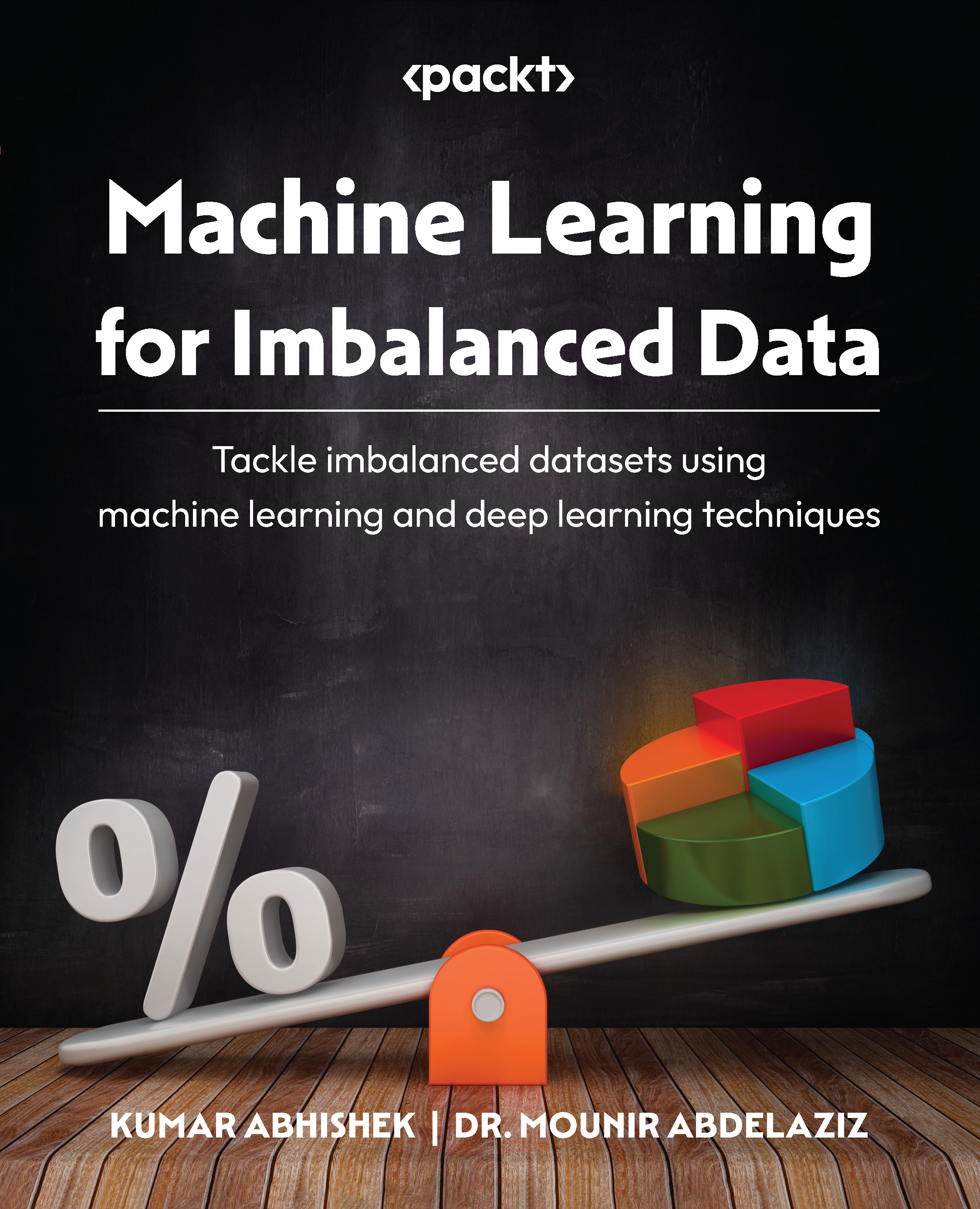
Machine Learning for Imbalanced Data
€37.99
Causal Inference and Discovery in Python
€29.99
Total 105.97 Stars icon
Banner background image

Table of Contents

16 Chapters
Part 1: Gradient Boosting and LightGBM Fundamentals Chevron down icon Chevron up icon
Chapter 1: Introducing Machine Learning Chevron down icon Chevron up icon
Chapter 2: Ensemble Learning – Bagging and Boosting Chevron down icon Chevron up icon
Chapter 3: An Overview of LightGBM in Python Chevron down icon Chevron up icon
Chapter 4: Comparing LightGBM, XGBoost, and Deep Learning Chevron down icon Chevron up icon
Part 2: Practical Machine Learning with LightGBM Chevron down icon Chevron up icon
Chapter 5: LightGBM Parameter Optimization with Optuna Chevron down icon Chevron up icon
Chapter 6: Solving Real-World Data Science Problems with LightGBM Chevron down icon Chevron up icon
Chapter 7: AutoML with LightGBM and FLAML Chevron down icon Chevron up icon
Part 3: Production-ready Machine Learning with LightGBM Chevron down icon Chevron up icon
Chapter 8: Machine Learning Pipelines and MLOps with LightGBM Chevron down icon Chevron up icon
Chapter 9: LightGBM MLOps with AWS SageMaker Chevron down icon Chevron up icon
Chapter 10: LightGBM Models with PostgresML Chevron down icon Chevron up icon
Chapter 11: Distributed and GPU-Based Learning with LightGBM Chevron down icon Chevron up icon
Index Chevron down icon Chevron up icon
Other Books You May Enjoy Chevron down icon Chevron up icon

Customer reviews

Top Reviews
Rating distribution
Full star icon Full star icon Full star icon Full star icon Half star icon 4.4
(8 Ratings)
5 star 62.5%
4 star 12.5%
3 star 25%
2 star 0%
1 star 0%
Filter icon Filter
Top Reviews

Filter reviews by


Om S Oct 10, 2023
Full star icon Full star icon Full star icon Full star icon Full star icon 5
"Machine Learning with LightGBM and Python" is a fantastic guide for both beginners and experienced folks. It introduces you to the powerful LightGBM framework, making machine learning easier. You'll learn about decision trees, gradient boosting, and more in simple language. The book takes you through practical case studies, so you can use machine learning to solve real problems.As you progress, you'll even learn how to build and scale your machine learning systems using tools like FastAPI and AWS Sagemaker. It's perfect for anyone who wants to improve their machine learning skills. You should know some Python, but you don't need to be an expert. This book is your key to understanding LightGBM and mastering machine learning.In short, it's a great book for those who want to excel in machine learning and build production-ready systems.
Amazon Verified review Amazon
H2N Oct 16, 2023
Full star icon Full star icon Full star icon Full star icon Full star icon 5
"Machine Learning with LightGBM and Python" is a detailed guide tailored for both newcomers and experts in machine learning. It sheds light on the LightGBM framework, emphasizing hands-on experience with key concepts like decision trees and gradient boosting. The book starts with foundational machine learning topics, then ventures into ensemble learning, showcasing algorithms like random forests. It prominently features LightGBM, comparing its strengths with other methods like XGBoost and deep neural networks. The text also explores hyperparameter optimization using Optuna, offers practical case studies, and introduces AutoML via FLAML. Transitioning from theory to application, it discusses ML pipelines, MLOps, AWS SageMaker, and harnessing distributed computing with LightGBM. This book is a comprehensive roadmap for mastering machine learning with Python and LightGBM.
Amazon Verified review Amazon
Amazon Customer Nov 09, 2023
Full star icon Full star icon Full star icon Full star icon Full star icon 5
The book strikes a good balance between theory and practical applications, ensuring that readers understand both the underlying principles and their real-world relevance. The code examples are well-structured and easy to follow, making it effortless for readers to implement the concepts discussed in the book. particularly appreciated the chapter on bagging and boosting which is the principle of LightGBM. The book also covers various evaluation metrics and hyperparameter tuning, providing readers with a comprehensive understanding of model optimization. While the book focuses on Light GBM, it also touches upon other important machine learning concepts, ensuring readers have a well-rounded understanding of the field.Overall, "Machine Learning with Light GBM and Python" is a valuable resource for anyone interested in leveraging the power of Light GBM in their machine learning projects. Whether you're a beginner or an experienced practitioner, this book will equip you with the knowledge and practical skills needed to excel in the field of machine learning.
Amazon Verified review Amazon
Sangita Mahala Nov 29, 2023
Full star icon Full star icon Full star icon Full star icon Full star icon 5
I strongly suggest this book for individuals who possess an interest in data, a proficiency in Python programming, and a curiosity to delve into the diverse realm of machine learning with LightGBM. It will undoubtedly enhance their skill set.
Amazon Verified review Amazon
Steven Fernandes Oct 29, 2023
Full star icon Full star icon Full star icon Full star icon Full star icon 5
This book offers a comprehensive introduction to machine learning (ML) with a focus on Python and scikit-learn. It guides readers through various ML techniques, including decision trees, ensemble learning, and advanced methods like gradient boosting, DART, and GOSS. Special attention is given to mastering LightGBM for both classification and regression challenges. The book also emphasizes the importance of AutoML tools like FLAML and Optuna for model optimization. Readers will learn to construct ML pipelines for efficient training and deployment, and how to scale their ML solutions using AWS Sagemaker, PostgresML, and Dask for production-level applications.
Amazon Verified review Amazon
Get free access to Packt library with over 7500+ books and video courses for 7 days!
Start Free Trial

FAQs

How do I buy and download an eBook? Chevron down icon Chevron up icon

Where there is an eBook version of a title available, you can buy it from the book details for that title. Add either the standalone eBook or the eBook and print book bundle to your shopping cart. Your eBook will show in your cart as a product on its own. After completing checkout and payment in the normal way, you will receive your receipt on the screen containing a link to a personalised PDF download file. This link will remain active for 30 days. You can download backup copies of the file by logging in to your account at any time.

If you already have Adobe reader installed, then clicking on the link will download and open the PDF file directly. If you don't, then save the PDF file on your machine and download the Reader to view it.

Please Note: Packt eBooks are non-returnable and non-refundable.

Packt eBook and Licensing When you buy an eBook from Packt Publishing, completing your purchase means you accept the terms of our licence agreement. Please read the full text of the agreement. In it we have tried to balance the need for the ebook to be usable for you the reader with our needs to protect the rights of us as Publishers and of our authors. In summary, the agreement says:

  • You may make copies of your eBook for your own use onto any machine
  • You may not pass copies of the eBook on to anyone else
How can I make a purchase on your website? Chevron down icon Chevron up icon

If you want to purchase a video course, eBook or Bundle (Print+eBook) please follow below steps:

  1. Register on our website using your email address and the password.
  2. Search for the title by name or ISBN using the search option.
  3. Select the title you want to purchase.
  4. Choose the format you wish to purchase the title in; if you order the Print Book, you get a free eBook copy of the same title. 
  5. Proceed with the checkout process (payment to be made using Credit Card, Debit Cart, or PayPal)
Where can I access support around an eBook? Chevron down icon Chevron up icon
  • If you experience a problem with using or installing Adobe Reader, the contact Adobe directly.
  • To view the errata for the book, see www.packtpub.com/support and view the pages for the title you have.
  • To view your account details or to download a new copy of the book go to www.packtpub.com/account
  • To contact us directly if a problem is not resolved, use www.packtpub.com/contact-us
What eBook formats do Packt support? Chevron down icon Chevron up icon

Our eBooks are currently available in a variety of formats such as PDF and ePubs. In the future, this may well change with trends and development in technology, but please note that our PDFs are not Adobe eBook Reader format, which has greater restrictions on security.

You will need to use Adobe Reader v9 or later in order to read Packt's PDF eBooks.

What are the benefits of eBooks? Chevron down icon Chevron up icon
  • You can get the information you need immediately
  • You can easily take them with you on a laptop
  • You can download them an unlimited number of times
  • You can print them out
  • They are copy-paste enabled
  • They are searchable
  • There is no password protection
  • They are lower price than print
  • They save resources and space
What is an eBook? Chevron down icon Chevron up icon

Packt eBooks are a complete electronic version of the print edition, available in PDF and ePub formats. Every piece of content down to the page numbering is the same. Because we save the costs of printing and shipping the book to you, we are able to offer eBooks at a lower cost than print editions.

When you have purchased an eBook, simply login to your account and click on the link in Your Download Area. We recommend you saving the file to your hard drive before opening it.

For optimal viewing of our eBooks, we recommend you download and install the free Adobe Reader version 9.