Why policy-based methods?
The objective of reinforcement learning is to find the optimal policy, which is the policy that provides the maximum return. So far, we have learned several different algorithms for computing the optimal policy, and all these algorithms have been value-based methods. Wait, what are value-based methods? Let's recap what value-based methods are, and the problems associated with them, and then we will learn about policy-based methods. Recapping is always good, isn't it?
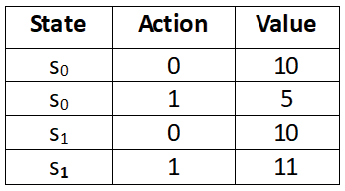
With value-based methods, we extract the optimal policy from the optimal Q function (Q values), meaning we compute the Q values of all state-action pairs to find the policy. We extract the policy by selecting an action in each state that has the maximum Q value. For instance, let's say we have two states s0 and s1 and our action space has two actions; let the actions be 0 and 1. First, we compute the Q value of all the state-action pairs, as shown in the following table. Now, we extract policy from the Q function (Q values) by selecting action 0 in state s0 and action 1 in state s1 as they have the maximum Q value:

Table 10.1: Q table
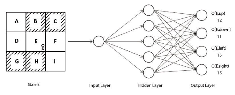
Later, we learned that it is difficult to compute the Q function when our environment has a large number of states and actions as it would be expensive to compute the Q values of all possible state-action pairs. So, we resorted to the Deep Q Network (DQN). In DQN, we used a neural network to approximate the Q function (Q value). Given a state, the network will return the Q values of all possible actions in that state. For instance, consider the grid world environment. Given a state, our DQN will return the Q values of all possible actions in that state. Then we select the action that has the highest Q value. As we can see in Figure 10.1, given state E, DQN returns the Q value of all possible actions (up, down, left, right). Then we select the right action in state E since it has the maximum Q value:

Figure 10.1: DQN
Thus, in value-based methods, we improve the Q function iteratively, and once we have the optimal Q function, then we extract optimal policy by selecting the action in each state that has the maximum Q value.
One of the disadvantages of the value-based method is that it is suitable only for discrete environments (environments with a discrete action space), and we cannot apply value-based methods in continuous environments (environments with a continuous action space).
We have learned that a discrete action space has a discrete set of actions; for example, the grid world environment has discrete actions (up, down, left, and right) and the continuous action space consists of actions that are continuous values, for example, controlling the speed of a car.
So far, we have only dealt with a discrete environment where we had a discrete action space, so we easily computed the Q value of all possible state-action pairs. But how can we compute the Q value of all possible state-action pairs when our action space is continuous? Say we are training an agent to drive a car and say we have one continuous action in our action space. Let the action be the speed of the car and the value of the speed of the car ranges from 0 to 150 kmph. In this case, how can we compute the Q value of all possible state-action pairs with the action being a continuous value?
In this case, we can discretize the continuous actions into speed (0 to 10) as action 1, speed (10 to 20) as action 2, and so on. After discretization, we can compute the Q value of all possible state-action pairs. However, discretization is not always desirable. We might lose several important features and we might end up in an action space with a huge set of actions.
Most real-world problems have continuous action space, say, a self-driving car, or a robot learning to walk and more. Apart from having a continuous action space they also have a high dimension. Thus, the DQN and other value-based methods cannot deal with the continuous action space effectively.
So, we use the policy-based methods. With policy-based methods, we don't need to compute the Q function (Q values) to find the optimal policy; instead, we can compute them directly. That is, we don't need the Q function to extract the policy. Policy-based methods have several advantages over value-based methods, and they can handle both discrete and continuous action spaces.
We learned that DQN takes care of the exploration-exploitation dilemma by using the epsilon-greedy policy. With the epsilon-greedy policy, we either select the best action with the probability 1-epsilon or a random action with the probability epsilon. Most policy-based methods use a stochastic policy. We know that with a stochastic policy, we select actions based on the probability distribution over the action space, which allows the agent to explore different actions instead of performing the same action every time. Thus, policy-based methods take care of the exploration-exploitation trade-off implicitly by using a stochastic policy. However, there are several policy-based methods that use a deterministic policy as well. We will learn more about them in the upcoming chapters.
Okay, how do policy-based methods work, exactly? How do they find an optimal policy without computing the Q function? We will learn about this in the next section. Now that we have a basic understanding of what a policy gradient method is, and also the disadvantages of value-based methods, in the next section we will learn about a fundamental and interesting policy-based method called policy gradient.


