Search icon CANCEL
Subscription
0
Cart icon
Your Cart (0 item)
Close icon
You have no products in your basket yet
Arrow left icon
Explore Products
Best Sellers
New Releases
Books
Videos
Audiobooks
Learning Hub
Newsletter Hub
Free Learning
Arrow right icon
timer SALE ENDS IN
0 Days
:
00 Hours
:
00 Minutes
:
00 Seconds
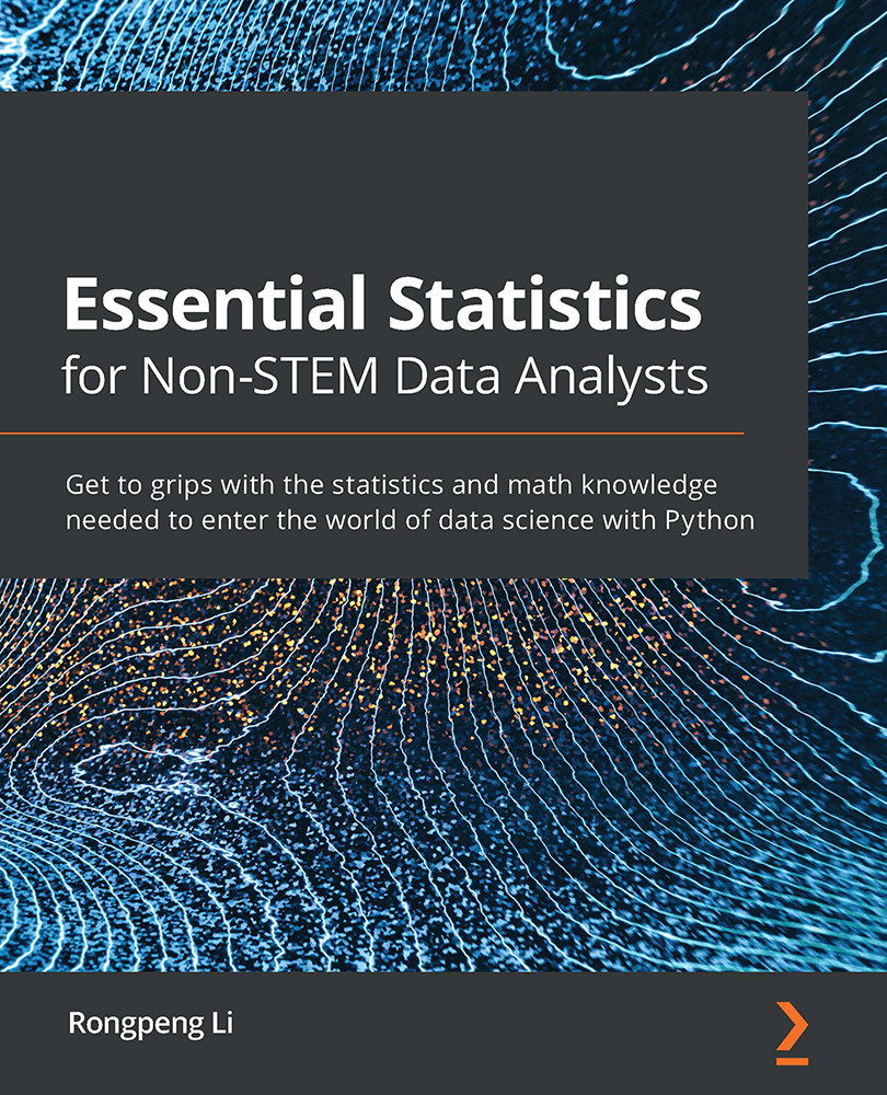
Essential Statistics for Non-STEM Data Analysts

Essential Statistics for Non-STEM Data Analysts: Get to grips with the statistics and math knowledge needed to enter the world of data science with Python

eBook
€17.99 €26.99
Paperback
€32.99
Subscription
Free Trial
Renews at €18.99p/m

What do you get with Print?

Product feature icon Instant access to your digital eBook copy whilst your Print order is Shipped
Product feature icon Paperback book shipped to your preferred address
Product feature icon Download this book in EPUB and PDF formats
Product feature icon Access this title in our online reader with advanced features
Product feature icon DRM FREE - Read whenever, wherever and however you want
Product feature icon AI Assistant (beta) to help accelerate your learning
OR
Modal Close icon
Payment Processing...
tick Completed

Shipping Address

Billing Address

Shipping Methods
Table of content icon View table of contents Preview book icon Preview Book

Essential Statistics for Non-STEM Data Analysts

Chapter 1: Fundamentals of Data Collection, Cleaning, and Preprocessing

Thank you for purchasing this book and welcome to a journal of exploration and excitement! Whether you are already a data scientist, preparing for an interview, or just starting learning, this book will serve you well as a companion. You may already be familiar with common Python toolkits and have followed trending tutorials online. However, there is a lack of a systematic approach to the statistical side of data science. This book is designed and written to close this gap for you.

As the first chapter in the book, we start with the very first step of a data science project: collecting, cleaning data, and performing some initial preprocessing. It is like preparing fish for cooking. You get the fish from the water or from the fish market, examine it, and process it a little bit before bringing it to the chef.

You are going to learn five key topics in this chapter. They are correlated with other topics, such as visualization and basic statistics concepts. For example, outlier removal will be very hard to conduct without a scatter plot. Data standardization clearly requires an understanding of statistics such as standard deviation. We prepared a GitHub repository that contains ready-to-run codes from this chapter as well as the rest.

Here are the topics that will be covered in this chapter:

  • Collecting data from various data sources with a focus on data quality
  • Data imputation with an assessment of downstream task requirements
  • Outlier removal
  • Data standardization – when and how
  • Examples involving the scikit-learn preprocessing module

The role of this chapter is as a primer. It is not possible to cover the topics in an entirely sequential fashion. For example, to remove outliers, necessary techniques such as statistical plotting, specifically a box plot and scatter plot, will be used. We will come back to those techniques in detail in future chapters of course, but you must bear with it now. Sometimes, in order to learn new topics, bootstrapping may be one of a few ways to break the shell. You will enjoy it because the more topics you learn along the way, the higher your confidence will be.

Technical requirements

The best environment for running the Python code in the book is on Google Colaboratory (https://colab.research.google.com). Google Colaboratory is a product that runs Jupyter Notebook in the cloud. It has common Python packages that are pre-installed and runs in a browser. It can also communicate with a disk so that you can upload local files to Google Drive. The recommended browsers are the latest versions of Chrome and Firefox.

For more information about Colaboratory, check out their official notebooks: https://colab.research.google.com .

You can find the code for this chapter in the following GitHub repository: https://github.com/PacktPublishing/Essential-Statistics-for-Non-STEM-Data-Analysts

Collecting data from various data sources

There are three major ways to collect and gather data. It is crucial to keep in mind that data doesn't have to be well-formatted tables:

  • Obtaining structured tabulated data directly: For example, the Federal Reserve (https://www.federalreserve.gov/data.htm) releases well-structured and well-documented data in various formats, including CSV, so that pandas can read the file into a DataFrame format.
  • Requesting data from an API: For example, the Google Map API (https://developers.google.com/maps/documentation) allows developers to request data from the Google API at a capped rate depending on the pricing plan. The returned format is usually JSON or XML.
  • Building a dataset from scratch: For example, social scientists often perform surveys and collect participants' answers to build proprietary data.

Let's look at some examples involving these three approaches. You will use the UCI machine learning repository, the Google Map API and USC President's Office websites as data sources, respectively.

Reading data directly from files

Reading data from local files or remote files through a URL usually requires a good source of publicly accessible data archives. For example, the University of California, Irvine maintains a data repository for machine learning. We will be reading the air quality dataset with pandas. The latest URL will be updated in the book's official GitHub repository in case the following code fails. You may obtain the file from https://archive.ics.uci.edu/ml/machine-learning-databases/heart-disease/. From the datasets, we are using the processed.hungarian.data file. You need to upload the file to the same folder where the notebook resides.

The following code snippet reads the data and displays the first several rows of the datasets:

import pandas as pd
df = pd.read_csv("processed.hungarian.data",
                 sep=",",
                 names = ["age","sex","cp","trestbps",
                          "chol","fbs","restecg","thalach",
                          "exang","oldpeak","slope","ca",
                          "thal","num"])
df.head()

This produces the following output:

Figure 1.1 – Head of the Hungarian heart disease dataset

Figure 1.1 – Head of the Hungarian heart disease dataset

In the following section, you will learn how to obtain data from an API.

Obtaining data from an API

In plain English, an Application Programming Interface (API) defines protocols, agreements, or treaties between applications or parts of applications. You need to pass requests to an API and obtain returned data in JSON or other formats specified in the API documentation. Then you can extract the data you want.

Note

When working with an API, you need to follow the guidelines and restrictions regarding API usage. Improper usage of an API will result in the suspension of an account or even legal issues.

Let's take the Google Map Place API as an example. The Place API (https://developers.google.com/places/web-service/intro) is one of many Google Map APIs that Google offers. Developers can use HTTP requests to obtain information about certain geographic locations, the opening hours of establishments, and the types of establishment, such as schools, government offices, and police stations.

In terms of using external APIs

Like many APIs, the Google Map Place API requires you to create an account on its platform – the Google Cloud Platform. It is free, but still requires a credit card account for some services it provides. Please pay attention so that you won't be mistakenly charged.

After obtaining and activating the API credentials, the developer can build standard HTTP requests to query the endpoints. For example, the textsearch endpoint is used to query places based on text. Here, you will use the API to query information about libraries in Culver City, Los Angeles:

  1. First, let's import the necessary libraries:
    import requests
    import json
  2. Initialize the API key and endpoints. We need to replace API_KEY with a real API key to make the code work:
    API_KEY = Your API key goes here
    TEXT_SEARCH_URL = https://maps.googleapis.com/maps/api/place/textsearch/json?
    query = "Culver City Library"
  3. Obtain the response returned and parse the returned data into JSON format. Let's examine it:
    response = requests.get(TEXT_SEARCH_URL+'query='+query+'&key='+API_KEY) 
    json_object = response.json() 
    print(json_object)

This is a one-result response. Otherwise, the results fields will have multiple entries. You can index the multi-entry results fields as a normal Python list object:

{'html_attributions': [],
 'results': [{'formatted_address': '4975 Overland Ave, Culver City, CA 90230, United States',
   'geometry': {'location': {'lat': 34.0075635, 'lng': -118.3969651},
    'viewport': {'northeast': {'lat': 34.00909257989272,
      'lng': -118.3955611701073},
     'southwest': {'lat': 34.00639292010727, 'lng': -118.3982608298927}}},
   'icon': 'https://maps.gstatic.com/mapfiles/place_api/icons/civic_building-71.png',
   'id': 'ccdd10b4f04fb117909897264c78ace0fa45c771',
   'name': 'Culver City Julian Dixon Library',
   'opening_hours': {'open_now': True},
   'photos': [{'height': 3024,
     'html_attributions': ['<a href="https://maps.google.com/maps/contrib/102344423129359752463">Khaled Alabed</a>'],
     'photo_reference': 'CmRaAAAANT4Td01h1tkI7dTn35vAkZhx_-mg3PjgKvjHiyh80M5UlI3wVw1cer4vkOksYR68NM9aw33ZPYGQzzXTE8bkOwQYuSChXAWlJUtz8atPhmRht4hP4dwFgqfbJULmG5f1EhAfWlF_cpLz76sD_81fns1OGhT4KU-zWTbuNY54_4_XozE02pLNWw',
     'width': 4032}],
   'place_id': 'ChIJrUqREx-6woARFrQdyscOZ-8',
   'plus_code': {'compound_code': '2J53+26 Culver City, California',
    'global_code': '85632J53+26'},
   'rating': 4.2,
   'reference': 'ChIJrUqREx-6woARFrQdyscOZ-8',
   'types': ['library', 'point_of_interest', 'establishment'],
   'user_ratings_total': 49}],
 'status': 'OK'}

The address and name of the library can be obtained as follows:

print(json_object["results"][0]["formatted_address"])
print(json_object["results"][0]["name"])

The result reads as follows:

4975 Overland Ave, Culver City, CA 90230, United States
Culver City Julian Dixon Library

Information

An API can be especially helpful for data augmentation. For example, if you have a list of addresses that are corrupted or mislabeled, using the Google Map API may help you correct wrong data.

Obtaining data from scratch

There are instances where you would need to build your own dataset from scratch.

One way of building data is to crawl and parse the internet. On the internet, a lot of public resources are open to the public and free to use. Google's spiders crawl the internet relentlessly 24/7 to keep its search results up to date. You can write your own code to gather information online instead of opening a web browser to do it manually.

Doing a survey and obtaining feedback, whether explicitly or implicitly, is another way to obtain private data. Companies such as Google and Amazon gather tons of data from user profiling. Such data builds the core of their dominating power in ads and e-commerce. We won't be covering this method, however.

Legal issue of crawling

Notice that in some cases, web crawling is highly controversial. Before crawling a website, do check their user agreement. Some websites explicitly forbid web crawling. Even if a website is open to web crawling, intensive requests may dramatically slow down the website, disabling its normal functionality to serve other users. It is a courtesy not only to respect their policy, but also the law.

Here is a simple example that uses regular expression to obtain all the phone numbers from the web page of the president's office, University of Southern California: http://departmentsdirectory.usc.edu/pres_off.html:

  1. First, let's import the necessary libraries. re is the Python built-in regular expression library. requests is an HTTP client that enables communication with the internet through the http protocol:
    import re
    import requests
  2. If you look at the web page, you will notice that there is a pattern within the phone numbers. All the phone numbers start with three digits, followed by a hyphen and then four digits. Our objective now is to compile such a pattern:
    pattern = re.compile("\d{3}-\d{4}")
  3. The next step is to create an http client and obtain the response from the GET call:
    response = requests.get("http://departmentsdirectory.usc.edu/pres_off.html") 
  4. The data attribute of response can be converted into a long string and fed to the findall method:
    pattern.findall(str(response.data))

The results contain all the phone numbers on the web page:

 ['740-2111',
 '821-1342',
 '740-2111',
 '740-2111',
 '740-2111',
 '740-2111',
 '740-2111',
 '740-2111',
 '740-9749',
 '740-2505',
 '740-6942',
 '821-1340',
 '821-6292']

In this section, we introduced three different ways of collecting data: reading tabulated data from data files provided by others, obtaining data from APIs, and building data from scratch. In the rest of the book, we will focus on the first option and mainly use collected data from the UCI Machine Learning Repository. In most cases, API data and scraped data will be integrated into tabulated datasets for production usage.

Data imputation

Missing data is ubiquitous and data imputation techniques will help us to alleviate its influence.

In this section, we are going to use the heart disease data to examine the pros and cons of basic data imputation. I recommend you read the dataset description beforehand to understand the meaning of each column.

Preparing the dataset for imputation

The heart disease dataset is the same one we used earlier in the Collecting data from various data sources section. It should give you a real red flag that you shouldn't take data integrity for granted. The following screenshot shows missing data denoted by question marks:

Figure 1.2 – The head of Hungarian heart disease data in VS Code (CSV rainbow extension enabled)

Figure 1.2 – The head of Hungarian heart disease data in VS Code (CSV rainbow extension enabled)

First, let's do an info() call that lists column data type information:

df.info()

Note

df.info() is a very helpful function that provides you with pointers for your next move. It should be the first function call when given an unknown dataset.

The following screenshot shows the output obtained from the preceding function:

Figure 1.3 – Output of the info() function call

Figure 1.3 – Output of the info() function call

If pandas can't infer the data type of a column, it will interpret it as objects. For example, the chol (cholesterol) column contains missing data. The missing data is a question mark treated as a string, but the remainder of the data is of the float type. The records are collectively called objects.

Python's type tolerance

As Python is pretty error-tolerant, it is a good practice to introduce a necessary type check. For example, if a column mixes the numerical values, instead of using numerical values to check truth, explicitly check its type and write two branches. Also, it is advised to avoid type conversion on columns with data type objects. Remember to make your code completely deterministic and future-proof.

Now, let's replace the question mark with the NaN values. The following code snippet declares a function that can handle three different cases and treat them appropriately. The three cases are listed here:

  • The record value is "?".
  • The record value is of the integer type. This is treated independently because columns such as num should be binary. Floating numbers will lose the essence of using 0-1 encoding.
  • The rest includes valid strings that can be converted to float numbers and original float numbers.

The code snippet will be as follows:

import numpy as np
def replace_question_mark(val):
    if val == "?":
        return np.NaN
    elif type(val)==int:
        return val
    else:
        return float(val)
df2 = df.copy()
for (columnName, _) in df2.iteritems():
    df2[columnName] = df2[columnName].apply(replace-question_mark)

Now we call the info() function and the head() function, as shown here:

df2.info()

You should expect that all fields are now either floats or integers, as shown in the following output:

Figure 1.4 – Output of info() after data type conversion

Figure 1.4 – Output of info() after data type conversion

Now you can check the number of non-null entries for each column, and different columns have different levels of completeness. age and sex don't contain missing values, but ca contains almost no valid data. This should guide you on your choices of data imputation. For example, strictly dropping all the missing values, which is also considered a way of data imputation, will almost remove the complete dataset. Let's check the shape of the DataFrame after the default missing value drops. You see that there is only one row left. We don't want it:

df2.dropna().shape

A screenshot of the output is as follows:

Figure 1.5 – Removing records containing NaN values leaves only one entry

Figure 1.5 – Removing records containing NaN values leaves only one entry

Before moving on to other more mainstream imputation methods, we would love to perform a quick review of our processed DataFrame.

Check the head of the new DataFrame. You should see that all question marks are replaced by NaN values. NaN values are treated as legitimate numerical values, so native NumPy functions can be used on them:

df2.head()

The output should look as follows:

Figure 1.6 – The head of the updated DataFrame

Figure 1.6 – The head of the updated DataFrame

Now, let's call the describe() function, which generates a table of statistics. It is a very helpful and handy function for a quick peak at common statistics in our dataset:

df2.describe()

Here is a screenshot of the output:

Figure 1.7 – Output from the describe() call

Figure 1.7 – Output from the describe() call

Understanding the describe() limitation

Note that the describe() function only considers valid values. In this sample, the average age value is more trustworthy than the average thal value. Do also pay attention to the metadata. A numerical value doesn't necessarily have a numerical meaning. For example, a thal value is encoded to integers with given meanings.

Now, let's examine the two most common ways of imputation.

Imputation with mean or median values

Imputation with mean or median values only works on numerical datasets. Categorical variables don't contain structures, such as one label being larger than another. Therefore, the concepts of mean and median won't apply.

There are several advantages associated with mean/median imputation:

  • It is easy to implement.
  • Mean/median imputation doesn't introduce extreme values.
  • It does not have any time limit.

However, there are some statistical consequences of mean/median imputation. The statistics of the dataset will change. For example, the histogram for cholesterol prior to imputation is provided here:

Figure 1.8 – Cholesterol concentration distribution

Figure 1.8 – Cholesterol concentration distribution

The following code snippet does the imputation with the mean. Following imputation the with mean, the histogram shifts to the right a little bit:

chol = df2["chol"]
plt.hist(chol.apply(lambda x: np.mean(chol) if np.isnan(x) else x), bins=range(0,630,30))
plt.xlabel("cholesterol imputation")
plt.ylabel("count")
Figure 1.9 – Cholesterol concentration distribution with mean imputation

Figure 1.9 – Cholesterol concentration distribution with mean imputation

Imputation with the median will shift the peak to the left because the median is smaller than the mean. However, it won't be obvious if you enlarge the bin size. Median and mean values will likely fall into the same bin in this eventuality:

Figure 1.10 – Cholesterol imputation with median imputation

Figure 1.10 – Cholesterol imputation with median imputation

The good news is that the shape of the distribution looks rather similar. The bad news is that we probably increased the level of concentration a little bit. We will cover such statistics in Chapter 3, Visualization with Statistical Graphs.

Note

In other cases where the distribution is not centered or contains a substantial ratio of missing data, such imputation can be disastrous. For example, if the waiting time in a restaurant follows an exponential distribution, imputation with mean values will probably break the characteristics of the distribution.

Imputation with the mode/most frequent value

The advantage of using the most frequent value is that it works well with categorical features and, without a doubt, it will introduce bias as well. The slope field is categorical in nature, although it looks numerical. It represents three statuses of a slope value as positive, flat, or negative.

The following code snippet will reveal our observation:

plt.hist(df2["slope"],bins = 5)
plt.xlabel("slope")
plt.ylabel("count");

Here is the output:

Figure 1.11 – Counting of the slope variable

Figure 1.11 – Counting of the slope variable

Without a doubt, the mode is 2. Following imputation with the mode, we obtain the following new distribution:

plt.hist(df2["slope"].apply(lambda x: 2 if np.isnan(x) else x),bins=5)
plt.xlabel("slope mode imputation")
plt.ylabel("count");

In the following graph, pay attention to the scale on y:

Figure 1.12 – Counting of the slope variable after mode imputation

Figure 1.12 – Counting of the slope variable after mode imputation

Replacing missing values with the mode in this case is disastrous. If positive and negative values of slope have medical consequences, performing prediction tasks on the preprocessed dataset will depress their weights and significance.

Different imputation methods have their own pros and cons. The prerequisite is to fully understand your business goals and downstream tasks. If key statistics are important, you should try to avoid distorting them. Also, do remember that collecting more data is always an option.

Outlier removal

Outliers can stem from two possibilities. They either come from mistakes or they have a story behind them. In principle, outliers should be very rare, otherwise the experiment/survey for generating the dataset is intrinsically flawed.

The definition of an outlier is tricky. Outliers can be legitimate because they fall into the long tail end of the population. For example, a team working on financial crisis prediction establishes that a financial crisis occurs in one out of 1,000 simulations. Of course, the result is not an outlier that should be discarded.

It is often good to keep original mysterious outliers from the raw data if possible. In other words, the reason to remove outliers should only come from outside the dataset – only when you already know the originals. For example, if the heart rate data is strangely fast and you know there is something wrong with the medical equipment, then you can remove the bad data. The fact that you know the sensor/equipment is wrong can't be deduced from the dataset itself.

Perhaps the best example for including outliers in data is the discovery of Neptune. In 1821, Alexis Bouvard discovered substantial deviations in Uranus' orbit based on observations. This led him to hypothesize that another planet may be affecting Uranus' orbit, which was found to be Neptune.

Otherwise, discarding mysterious outliers is risky for downstream tasks. For example, some regression tasks are sensitive to extreme values. It takes further experiments to decide whether the outliers exist for a reason. In such cases, don't remove or correct outliers in the data preprocessing steps.

The following graph generates a scatter plot for the trestbps and chol fields. The highlighted data points are possible outliers, but I probably will keep them for now:

Figure 1.13 – A scatter plot of two fields in heart disease dataset

Figure 1.13 – A scatter plot of two fields in heart disease dataset

Like missing data imputation, outlier removal is tricky and depends on the quality of data and your understanding of the data.

It is hard to discuss systemized outlier removal without talking about concepts such as quartiles and box plots. In this section, we looked at the background information pertaining to outlier removal. We will talk about the implementation based on statistical criteria in the corresponding sections in Chapter 2, Essential Statistics for Data Assessment, and Chapter 3, Visualization with Statistical Graphs.

Data standardization – when and how

Data standardization is a common preprocessing step. I use the terms standardization and normalization interchangeably. You may also encounter the concept of rescaling in literature or blogs.

Standardization often means shifting the data to be zero-centered with a standard deviation of 1. The goal is to bring variables with different units/ranges down to the same range. Many machine learning tasks are sensitive to data magnitudes. Standardization is supposed to remove such factors.

Rescaling doesn't necessarily bring the variables to a common range. This is done by means of customized mapping, usually linear, to scale original data to a different range. However, the common approach of min-max scaling does transform different variables into a common range [0, 1].

People may argue about the difference between standardization and normalization. When comparing their differences, normalization will refer to normalizing different variables to the same range [0, 1], and min-max scaling is considered a normalization algorithm. However, there are other normalization algorithms as well. Standardization cares more about the mean and standard deviation.

Standardization also transforms the original distribution closer to a Gaussian distribution. In the event that the original distribution is indeed Gaussian, standardization outputs a standard Gaussian distribution.

When to perform standardization

Perform standardization when your downstream tasks require it. For example, the k-nearest neighbors method is sensitive to variable magnitudes, so you should standardize the data. On the other hand, tree-based methods are not sensitive to different ranges of variables, so standardization is not required.

There are mature libraries to perform standardization. We first calculate the standard deviation and mean of the data, subtract the mean from every entry, and then divide by the standard deviation. Standard deviation describes the level of variety in data that will be discussed more in Chapter 2, Essential Statistics for Data Assessment.

Here is an example involving vanilla Python:

stdChol = np.std(chol)
meanChol = np.mean(chol)
chol2 = chol.apply(lambda x: (x-meanChol)/stdChol)
plt.hist(chol2,bins=range(int(min(chol2)), int(max(chol2))+1, 1));

The output is as follows:

Figure 1.14 – Standardized cholesterol data

Figure 1.14 – Standardized cholesterol data

Note that the standardized distribution looks more like a Gaussian distribution now.

Data standardization is irreversible. Information will be lost in standardization. It is only recommended to do so when no original information, such as magnitudes or original standard deviation, will be required later. In most cases, standardization is a safe choice for most downstream data science tasks.

In the next section, we will use the scikit-learn preprocessing module to demonstrate tasks involving standardization.

Examples involving the scikit-learn preprocessing module

For both imputation and standardization, scikit-learn offers similar APIs:

  1. First, fit the data to learn the imputer or standardizer.
  2. Then, use the fitted object to transform new data.

In this section, I will demonstrate two examples, one for imputation and another for standardization.

Note

Scikit-learn uses the same syntax of fit and predict for predictive models. This is a very good practice for keeping the interface consistent. We will cover the machine learning methods in later chapters.

Imputation

First, create an imputer from the SimpleImputer class. The initialization of the instance allows you to choose missing value forms. It is handy as we can feed our original data into it by treating the question mark as a missing value:

from sklearn.impute import SimpleImputer
imputer = SimpleImputer(missing_values=np.nan, strategy="mean")

Note that fit and transform can accept the same input:

imputer.fit(df2)
df3 = pd.DataFrame(imputer.transform(df2))

Now, check the number of missing values – the result should be 0:

np.sum(np.sum(np.isnan(df3)))

Standardization

Standardization can be implemented in a similar fashion:

from sklearn import preprocessing

The scale function provides the default zero-mean, one-standard deviation transformation:

df4 = pd.DataFrame(preprocessing.scale(df2))

Note

In this example, categorical variables represented by integers are also zero-mean, which should be avoided in production.

Let's check the standard deviation and mean. The following line outputs infinitesimal values:

df4.mean(axis=0)

The following line outputs values close to 1:

df4.std(axis=0)

Let's look at an example of MinMaxScaler, which transforms every variable into the range [0, 1]. The following code fits and transforms the heart disease dataset in one step. It is left to you to examine its validity:

minMaxScaler = preprocessing.MinMaxScaler()
df5 = pd.DataFrame(minMaxScaler.fit_transform(df2))

Let's now summarize what we have learned in this chapter.

Summary

In this chapter, we covered several important topics that usually emerge at the earliest stage of a data science project. We examined their applicable scenarios and conservatively checked some consequences, either numerically or visually. Many arguments made here will be more prominent when we cover other more sophisticated topics later.

In the next chapter, we will review probabilities and statistical concepts, including the mean, the median, quartiles, standard deviation, and skewness. I am sure you will then have a deeper understanding of concepts such as outliers.

Left arrow icon Right arrow icon
Download code icon Download Code

Key benefits

  • Work your way through the entire data analysis pipeline with statistics concerns in mind to make reasonable decisions
  • Understand how various data science algorithms function
  • Build a solid foundation in statistics for data science and machine learning using Python-based examples

Description

Statistics remain the backbone of modern analysis tasks, helping you to interpret the results produced by data science pipelines. This book is a detailed guide covering the math and various statistical methods required for undertaking data science tasks. The book starts by showing you how to preprocess data and inspect distributions and correlations from a statistical perspective. You’ll then get to grips with the fundamentals of statistical analysis and apply its concepts to real-world datasets. As you advance, you’ll find out how statistical concepts emerge from different stages of data science pipelines, understand the summary of datasets in the language of statistics, and use it to build a solid foundation for robust data products such as explanatory models and predictive models. Once you’ve uncovered the working mechanism of data science algorithms, you’ll cover essential concepts for efficient data collection, cleaning, mining, visualization, and analysis. Finally, you’ll implement statistical methods in key machine learning tasks such as classification, regression, tree-based methods, and ensemble learning. By the end of this Essential Statistics for Non-STEM Data Analysts book, you’ll have learned how to build and present a self-contained, statistics-backed data product to meet your business goals.

Who is this book for?

This book is an entry-level guide for data science enthusiasts, data analysts, and anyone starting out in the field of data science and looking to learn the essential statistical concepts with the help of simple explanations and examples. If you’re a developer or student with a non-mathematical background, you’ll find this book useful. Working knowledge of the Python programming language is required.

What you will learn

  • Find out how to grab and load data into an analysis environment
  • Perform descriptive analysis to extract meaningful summaries from data
  • Discover probability, parameter estimation, hypothesis tests, and experiment design best practices
  • Get to grips with resampling and bootstrapping in Python
  • Delve into statistical tests with variance analysis, time series analysis, and A/B test examples
  • Understand the statistics behind popular machine learning algorithms
  • Answer questions on statistics for data scientist interviews
Estimated delivery fee Deliver to Greece

Premium delivery 7 - 10 business days

€17.95
(Includes tracking information)

Product Details

Country selected
Publication date, Length, Edition, Language, ISBN-13
Publication date : Nov 12, 2020
Length: 392 pages
Edition : 1st
Language : English
ISBN-13 : 9781838984847
Category :
Languages :
Concepts :

What do you get with Print?

Product feature icon Instant access to your digital eBook copy whilst your Print order is Shipped
Product feature icon Paperback book shipped to your preferred address
Product feature icon Download this book in EPUB and PDF formats
Product feature icon Access this title in our online reader with advanced features
Product feature icon DRM FREE - Read whenever, wherever and however you want
Product feature icon AI Assistant (beta) to help accelerate your learning
OR
Modal Close icon
Payment Processing...
tick Completed

Shipping Address

Billing Address

Shipping Methods
Estimated delivery fee Deliver to Greece

Premium delivery 7 - 10 business days

€17.95
(Includes tracking information)

Product Details

Publication date : Nov 12, 2020
Length: 392 pages
Edition : 1st
Language : English
ISBN-13 : 9781838984847
Category :
Languages :
Concepts :

Packt Subscriptions

See our plans and pricing
Modal Close icon
€18.99 billed monthly
Feature tick icon Unlimited access to Packt's library of 7,000+ practical books and videos
Feature tick icon Constantly refreshed with 50+ new titles a month
Feature tick icon Exclusive Early access to books as they're written
Feature tick icon Solve problems while you work with advanced search and reference features
Feature tick icon Offline reading on the mobile app
Feature tick icon Simple pricing, no contract
€189.99 billed annually
Feature tick icon Unlimited access to Packt's library of 7,000+ practical books and videos
Feature tick icon Constantly refreshed with 50+ new titles a month
Feature tick icon Exclusive Early access to books as they're written
Feature tick icon Solve problems while you work with advanced search and reference features
Feature tick icon Offline reading on the mobile app
Feature tick icon Choose a DRM-free eBook or Video every month to keep
Feature tick icon PLUS own as many other DRM-free eBooks or Videos as you like for just €5 each
Feature tick icon Exclusive print discounts
€264.99 billed in 18 months
Feature tick icon Unlimited access to Packt's library of 7,000+ practical books and videos
Feature tick icon Constantly refreshed with 50+ new titles a month
Feature tick icon Exclusive Early access to books as they're written
Feature tick icon Solve problems while you work with advanced search and reference features
Feature tick icon Offline reading on the mobile app
Feature tick icon Choose a DRM-free eBook or Video every month to keep
Feature tick icon PLUS own as many other DRM-free eBooks or Videos as you like for just €5 each
Feature tick icon Exclusive print discounts

Frequently bought together


Stars icon
Total 115.97
Practical Discrete Mathematics
€49.99
Hands-On Mathematics for Deep Learning
€32.99
Essential Statistics for Non-STEM Data Analysts
€32.99
Total 115.97 Stars icon

Table of Contents

18 Chapters
Section 1: Getting Started with Statistics for Data Science Chevron down icon Chevron up icon
Chapter 1: Fundamentals of Data Collection, Cleaning, and Preprocessing Chevron down icon Chevron up icon
Chapter 2: Essential Statistics for Data Assessment Chevron down icon Chevron up icon
Chapter 3: Visualization with Statistical Graphs Chevron down icon Chevron up icon
Section 2: Essentials of Statistical Analysis Chevron down icon Chevron up icon
Chapter 4: Sampling and Inferential Statistics Chevron down icon Chevron up icon
Chapter 5: Common Probability Distributions Chevron down icon Chevron up icon
Chapter 6: Parametric Estimation Chevron down icon Chevron up icon
Chapter 7: Statistical Hypothesis Testing Chevron down icon Chevron up icon
Section 3: Statistics for Machine Learning Chevron down icon Chevron up icon
Chapter 8: Statistics for Regression Chevron down icon Chevron up icon
Chapter 9: Statistics for Classification Chevron down icon Chevron up icon
Chapter 10: Statistics for Tree-Based Methods Chevron down icon Chevron up icon
Chapter 11: Statistics for Ensemble Methods Chevron down icon Chevron up icon
Section 4: Appendix Chevron down icon Chevron up icon
Chapter 12: A Collection of Best Practices Chevron down icon Chevron up icon
Chapter 13: Exercises and Projects Chevron down icon Chevron up icon
Other Books You May Enjoy Chevron down icon Chevron up icon

Customer reviews

Top Reviews
Rating distribution
Full star icon Full star icon Full star icon Full star icon Half star icon 4.6
(10 Ratings)
5 star 70%
4 star 20%
3 star 10%
2 star 0%
1 star 0%
Filter icon Filter
Top Reviews

Filter reviews by


Amazon Customer Jan 05, 2021
Full star icon Full star icon Full star icon Full star icon Full star icon 5
I came to this book with the perspective of a non-STEM professional who is transitioning into a Data Science career - so it seemed like it could be an ideal resource for someone with my profile, and that is indeed the case!Previously, I had worked through online courses to learn some Python and some statistics, and had also used the books ‘Python the Hard Way’ and ‘Statistics for Dummies’ quite extensively. The challenge with both of those books is that, in order to become a working data analyst or data scientist, you really need to learn both topics hand-in-hand: it's best to learn statistics while also learning to code in Python. That's exactly what you get in THIS book - working through the essential mathematics/statistics concepts, and learning to code them as you go.These are tough subjects to learn and it's not easy for anyone who doesn't have previous experience in coding - as the author says early on in the book, for a few chapters it's best to just "code along" with the assignments even if you don't fully understand. As you become more familiar with Python, the syntax will start to make sense.Additional notes:- If you’re apprehensive about starting your data analysis/data science journey, this book includes a very clear explanation of how beginners can start coding (using Google Colabs or Jupyter Notebook).- There’s a full section on machine learning - this is what many people consider the most fun part of data science. Spend a lot of time and effort on the earlier sections of the book, and you’ll be fully ready to jump into the machine learning chapters.- Don’t miss the great chapter towards the end of the book, titled “A Collection of Best Practices” - it covers some of the ethical challenges of working with data, ranging from the publication of misleading graphs to the controversial use of facial recognition technology.
Amazon Verified review Amazon
Rongyu Lin May 22, 2021
Full star icon Full star icon Full star icon Full star icon Full star icon 5
It contains the most important knowledge that data analysts use in the daily work. Well organized and easy to understand. I would recommend this book to all my friends.
Amazon Verified review Amazon
data analyst Feb 23, 2021
Full star icon Full star icon Full star icon Full star icon Full star icon 5
This book is great for the beginner data analyst wanting to learn statistics and Python. Unlike some other statistics texts I have read, the examples are laid out with very simple python code without skipping the beginning steps. The preface even shows you how to install, import and read in an excel file with Pandas. All the example plots have their source code next to them which is extremely helpful to the beginner as well. Another important concept covered in this book is Data Preprocessing. It’s not all you will need to know but it is a great start. As an analyst, %80 of my time is spent on data preprocessing.
Amazon Verified review Amazon
Elsa V. Jan 27, 2021
Full star icon Full star icon Full star icon Full star icon Full star icon 5
I wish I'd had this book from the beginning of my journey. The graphics make it very easy to understand what we are talking about and the code is broken down and functional enough to make it easy and clear to understand the point. Li has the insight and clarity to teach data science in a way that even a 5 year old could understand. Absolutely recommend his book, for both stem and non-stem majors. (I have taken Data Sci at a prestigious school via the comp sci/engineering dept, completed a Data Sci bootcamp and work as a software engineer supporting a Data Sci team, and am a former kindergarten teacher and can professionally attest to the quality of digestibility of the info and the breadth and depth of topics.)
Amazon Verified review Amazon
Imran Sarker Feb 15, 2021
Full star icon Full star icon Full star icon Full star icon Full star icon 5
This book provides a lot of knowledge related to data analysis to its readers. It doesn’t matter whatyour background is when you read this book you start walking on the path to becoming a data analyst.Being an Analyst, it’s important to be familiar with Statistics in order to come up with results and turnyour idea into reality.Although, with the time being, new ways are being introduced but getting familiar with thebackground of everything is important. The author has distributed all the topics well so people fromany background a non-stem or stem can go through each chapter and learn as much as they can. Iwould definitely recommend this book to all who want to manage the data and find ways to deal with the data.
Amazon Verified review Amazon
Get free access to Packt library with over 7500+ books and video courses for 7 days!
Start Free Trial

FAQs

What is the delivery time and cost of print book? Chevron down icon Chevron up icon

Shipping Details

USA:

'

Economy: Delivery to most addresses in the US within 10-15 business days

Premium: Trackable Delivery to most addresses in the US within 3-8 business days

UK:

Economy: Delivery to most addresses in the U.K. within 7-9 business days.
Shipments are not trackable

Premium: Trackable delivery to most addresses in the U.K. within 3-4 business days!
Add one extra business day for deliveries to Northern Ireland and Scottish Highlands and islands

EU:

Premium: Trackable delivery to most EU destinations within 4-9 business days.

Australia:

Economy: Can deliver to P. O. Boxes and private residences.
Trackable service with delivery to addresses in Australia only.
Delivery time ranges from 7-9 business days for VIC and 8-10 business days for Interstate metro
Delivery time is up to 15 business days for remote areas of WA, NT & QLD.

Premium: Delivery to addresses in Australia only
Trackable delivery to most P. O. Boxes and private residences in Australia within 4-5 days based on the distance to a destination following dispatch.

India:

Premium: Delivery to most Indian addresses within 5-6 business days

Rest of the World:

Premium: Countries in the American continent: Trackable delivery to most countries within 4-7 business days

Asia:

Premium: Delivery to most Asian addresses within 5-9 business days

Disclaimer:
All orders received before 5 PM U.K time would start printing from the next business day. So the estimated delivery times start from the next day as well. Orders received after 5 PM U.K time (in our internal systems) on a business day or anytime on the weekend will begin printing the second to next business day. For example, an order placed at 11 AM today will begin printing tomorrow, whereas an order placed at 9 PM tonight will begin printing the day after tomorrow.


Unfortunately, due to several restrictions, we are unable to ship to the following countries:

  1. Afghanistan
  2. American Samoa
  3. Belarus
  4. Brunei Darussalam
  5. Central African Republic
  6. The Democratic Republic of Congo
  7. Eritrea
  8. Guinea-bissau
  9. Iran
  10. Lebanon
  11. Libiya Arab Jamahriya
  12. Somalia
  13. Sudan
  14. Russian Federation
  15. Syrian Arab Republic
  16. Ukraine
  17. Venezuela
What is custom duty/charge? Chevron down icon Chevron up icon

Customs duty are charges levied on goods when they cross international borders. It is a tax that is imposed on imported goods. These duties are charged by special authorities and bodies created by local governments and are meant to protect local industries, economies, and businesses.

Do I have to pay customs charges for the print book order? Chevron down icon Chevron up icon

The orders shipped to the countries that are listed under EU27 will not bear custom charges. They are paid by Packt as part of the order.

List of EU27 countries: www.gov.uk/eu-eea:

A custom duty or localized taxes may be applicable on the shipment and would be charged by the recipient country outside of the EU27 which should be paid by the customer and these duties are not included in the shipping charges been charged on the order.

How do I know my custom duty charges? Chevron down icon Chevron up icon

The amount of duty payable varies greatly depending on the imported goods, the country of origin and several other factors like the total invoice amount or dimensions like weight, and other such criteria applicable in your country.

For example:

  • If you live in Mexico, and the declared value of your ordered items is over $ 50, for you to receive a package, you will have to pay additional import tax of 19% which will be $ 9.50 to the courier service.
  • Whereas if you live in Turkey, and the declared value of your ordered items is over € 22, for you to receive a package, you will have to pay additional import tax of 18% which will be € 3.96 to the courier service.
How can I cancel my order? Chevron down icon Chevron up icon

Cancellation Policy for Published Printed Books:

You can cancel any order within 1 hour of placing the order. Simply contact customercare@packt.com with your order details or payment transaction id. If your order has already started the shipment process, we will do our best to stop it. However, if it is already on the way to you then when you receive it, you can contact us at customercare@packt.com using the returns and refund process.

Please understand that Packt Publishing cannot provide refunds or cancel any order except for the cases described in our Return Policy (i.e. Packt Publishing agrees to replace your printed book because it arrives damaged or material defect in book), Packt Publishing will not accept returns.

What is your returns and refunds policy? Chevron down icon Chevron up icon

Return Policy:

We want you to be happy with your purchase from Packtpub.com. We will not hassle you with returning print books to us. If the print book you receive from us is incorrect, damaged, doesn't work or is unacceptably late, please contact Customer Relations Team on customercare@packt.com with the order number and issue details as explained below:

  1. If you ordered (eBook, Video or Print Book) incorrectly or accidentally, please contact Customer Relations Team on customercare@packt.com within one hour of placing the order and we will replace/refund you the item cost.
  2. Sadly, if your eBook or Video file is faulty or a fault occurs during the eBook or Video being made available to you, i.e. during download then you should contact Customer Relations Team within 14 days of purchase on customercare@packt.com who will be able to resolve this issue for you.
  3. You will have a choice of replacement or refund of the problem items.(damaged, defective or incorrect)
  4. Once Customer Care Team confirms that you will be refunded, you should receive the refund within 10 to 12 working days.
  5. If you are only requesting a refund of one book from a multiple order, then we will refund you the appropriate single item.
  6. Where the items were shipped under a free shipping offer, there will be no shipping costs to refund.

On the off chance your printed book arrives damaged, with book material defect, contact our Customer Relation Team on customercare@packt.com within 14 days of receipt of the book with appropriate evidence of damage and we will work with you to secure a replacement copy, if necessary. Please note that each printed book you order from us is individually made by Packt's professional book-printing partner which is on a print-on-demand basis.

What tax is charged? Chevron down icon Chevron up icon

Currently, no tax is charged on the purchase of any print book (subject to change based on the laws and regulations). A localized VAT fee is charged only to our European and UK customers on eBooks, Video and subscriptions that they buy. GST is charged to Indian customers for eBooks and video purchases.

What payment methods can I use? Chevron down icon Chevron up icon

You can pay with the following card types:

  1. Visa Debit
  2. Visa Credit
  3. MasterCard
  4. PayPal
What is the delivery time and cost of print books? Chevron down icon Chevron up icon

Shipping Details

USA:

'

Economy: Delivery to most addresses in the US within 10-15 business days

Premium: Trackable Delivery to most addresses in the US within 3-8 business days

UK:

Economy: Delivery to most addresses in the U.K. within 7-9 business days.
Shipments are not trackable

Premium: Trackable delivery to most addresses in the U.K. within 3-4 business days!
Add one extra business day for deliveries to Northern Ireland and Scottish Highlands and islands

EU:

Premium: Trackable delivery to most EU destinations within 4-9 business days.

Australia:

Economy: Can deliver to P. O. Boxes and private residences.
Trackable service with delivery to addresses in Australia only.
Delivery time ranges from 7-9 business days for VIC and 8-10 business days for Interstate metro
Delivery time is up to 15 business days for remote areas of WA, NT & QLD.

Premium: Delivery to addresses in Australia only
Trackable delivery to most P. O. Boxes and private residences in Australia within 4-5 days based on the distance to a destination following dispatch.

India:

Premium: Delivery to most Indian addresses within 5-6 business days

Rest of the World:

Premium: Countries in the American continent: Trackable delivery to most countries within 4-7 business days

Asia:

Premium: Delivery to most Asian addresses within 5-9 business days

Disclaimer:
All orders received before 5 PM U.K time would start printing from the next business day. So the estimated delivery times start from the next day as well. Orders received after 5 PM U.K time (in our internal systems) on a business day or anytime on the weekend will begin printing the second to next business day. For example, an order placed at 11 AM today will begin printing tomorrow, whereas an order placed at 9 PM tonight will begin printing the day after tomorrow.


Unfortunately, due to several restrictions, we are unable to ship to the following countries:

  1. Afghanistan
  2. American Samoa
  3. Belarus
  4. Brunei Darussalam
  5. Central African Republic
  6. The Democratic Republic of Congo
  7. Eritrea
  8. Guinea-bissau
  9. Iran
  10. Lebanon
  11. Libiya Arab Jamahriya
  12. Somalia
  13. Sudan
  14. Russian Federation
  15. Syrian Arab Republic
  16. Ukraine
  17. Venezuela