Multiple Regression Analysis
In the exercises and activity so far, we have used only one independent variable in our regression analysis. In practice, as we have seen with the Boston Housing dataset, processes and phenomena of analytic interest are rarely influenced by only one feature. To be able to model the variability to a higher level of accuracy, therefore, it is necessary to investigate all the independent variables that may contribute significantly toward explaining the variability in the dependent variable. Multiple regression analysis is the method that is used to achieve this.
Exercise 2.05: Fitting a Multiple Linear Regression Model Using the Statsmodels Formula API
In this exercise, we will be using the plus operator (+) in the patsy formula string to define a linear regression model that includes more than one independent variable.
To complete this activity, run the code in the following steps in your Colab notebook:
- Open a new Colab notebook file and import the required packages.
import statsmodels.formula.api as smf
import pandas as pd
from sklearn.model_selection import train_test_split
- Execute Step 2 to 11 from Exercise 2.01, Loading and Preparing the Data for Analysis.
- Use the plus operator (
+) of the Patsy formula language to define a linear model that regressescrimeRatePerCapitaonpctLowerStatus,radialHighwaysAccess,medianValue_Ks, andnitrixOxide_pp10mand assign it to a variable namedmultiLinearModel. Use the Python line continuation symbol (\) to continue your code on a new line should you run out of space:multiLinearModel = smf.ols\ (formula = 'crimeRatePerCapita \ ~ pctLowerStatus \ + radialHighwaysAccess \ + medianValue_Ks \ + nitrixOxide_pp10m', \ data=train_data)
- Call the
fitmethod of the model instance and assign the results of the method to a variable:multiLinearModResult = multiLinearModel.fit()
- Print a summary of the results stored the variable created in Step 3:
print(multiLinearModResult.summary())
The output is as follows:
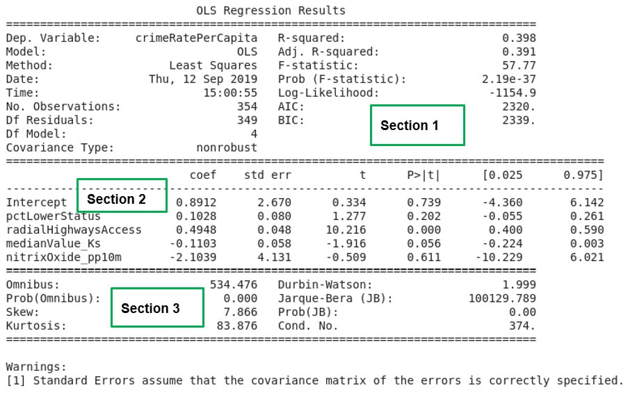
Figure 2.18: A summary of multiple linear regression results
Note
To access the source code for this specific section, please refer to https://packt.live/34cJgOK.
You can also run this example online at https://packt.live/3h1CKOt.
If the exercise was correctly followed, Figure 2.18 will be the result of the analysis. In Activity 2.01, the R-squared statistic was used to assess the model for goodness of fit. When multiple independent variables are involved, the goodness of fit of the model created is assessed using the adjusted R-squared statistic.
The adjusted R-squared statistic considers the presence of the extra independent variables in the model and corrects for inflation of the goodness of fit measure of the model, which is just caused by the fact that more independent variables are being used to create the model.
The lesson we learn from this exercise is the improvement in the adjusted R-squared value in Section 1 of Figure 2.18. When only one independent variable was used to create a model that seeks to explain the variability in crimeRatePerCapita in Exercise 2.04, Fitting a Simple Linear Regression Model Using the Statsmodels formula API, the R-squared value calculated was only 14.4 percent. In this exercise, we used four independent variables. The model that was created improved the adjusted R-squared statistic to 39.1 percent, an increase of 24.7 percent.
We learn that the presence of independent variables that are correlated to a dependent variable can help explain the variability in the independent variable in a model. But it is clear that a considerable amount of variability, about 60.9 percent, in the dependent variable is still not explained by our model.
There is still room for improvement if we want a model that does a good job of explaining the variability we see in crimeRatePerCapita. In Section 2 of Figure 2.18, the intercept and all the independent variables in our model are listed together with their coefficients. If we denote pctLowerStatus by x1, radialHighwaysAccess by x2, medianValue_Ks by x3 , and nitrixOxide_pp10m by x4, a mathematical expression for the model created can be written as y ≈ 0.8912+0.1028x1+0.4948x2-0.1103x3-2.1039x4.
The expression just stated defines the model created in this exercise, and it is comparable to the expression for multiple linear regression provided in Figure 2.5 earlier.


