Understanding the Data

In this first part, we load the data and perform an initial exploration of it.

Note

You can download the data either from the original source (https://archive.ics.uci.edu/ml/datasets/Bike+Sharing+Dataset#) or from the GitHub repository of this book (https://packt.live/2XpHW81).

The main goal of the presented steps is to acquire some basic knowledge about the data, how the various features are distributed, and whether there are missing values in it.

First import the relevant Python libraries and the data itself for the analysis. Note that we are using Python 3.7. Furthermore, we directly load the data from the GitHub repository of the book:

# imports
import pandas as pd
import seaborn as sns
import matplotlib.pyplot as plt
import numpy as np
%matplotlib inline
# load hourly data
hourly_data = pd.read_csv('https://raw.githubusercontent.com/'\
                          'PacktWorkshops/'\
                          'The-Data-Analysis-Workshop/'\
                          'master/Chapter01/data/hour.csv')

Note

The # symbol in the code snippet above denotes a code comment. Comments are added into code to help explain specific bits of logic. Also, watch out for the slashes in the string above. The backslashes ( \ ) are used to split the code across multiple lines, while the forward slashes ( / ) are part of the URL.

A good practice is to check the size of the data we are loading, the number of missing values of each column, and some general statistics about the numerical columns:

# print some generic statistics about the data
print(f"Shape of data: {hourly_data.shape}")
print(f"Number of missing values in the data:\
{hourly_data.isnull().sum().sum()}")

Note

The code snippet shown here uses a backslash ( \ ) to split the logic across multiple lines. When the code is executed, Python will ignore the backslash, and treat the code on the next line as a direct continuation of the current line.

The output is as follows:

Shape of data: (17379, 17)
Number of missing values in the data: 0

In order to get some simple statistics on the numerical columns, such as the mean, standard deviation, minimum and maximum values, and their percentiles, we can use the describe() function directly on a pandas.Dataset object:

# get statistics on the numerical columns
hourly_data.describe().T

The output should be as follows:

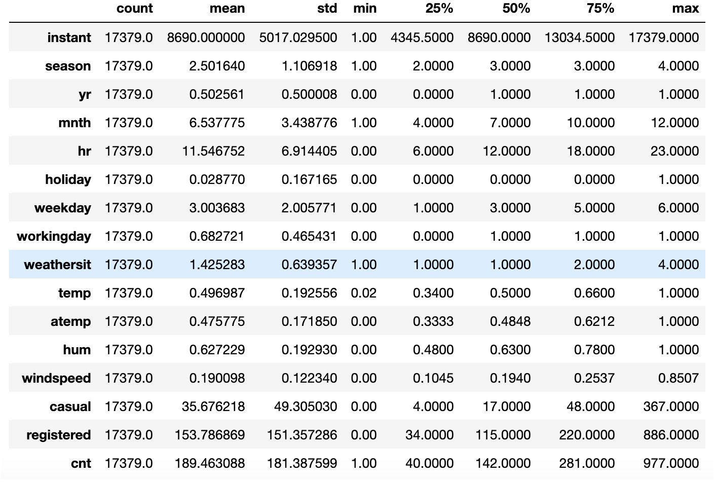
Figure 1.1: Output of the describe() method

Note that the T character after the describe() method gets the transpose of the resulting dataset, hence the columns become rows and vice versa.

According to the description of the original data, provided in the Readme.txt file, we can split the columns into three main groups:

• temporal features: This contains information about the time at which the record was registered. This group contains the dteday, season, yr, mnth, hr, holiday, weekday, and workingday columns.
• weather related features: This contains information about the weather conditions. The weathersit, temp, atemp, hum, and windspeed columns are included in this group.
• record related features: This contains information about the number of records for the specific hour and date. This group includes the casual, registered, and cnt columns.

Note that we did not include the first column, instant, in any of the previously mentioned groups. The reason for this is that it is an index column and will be excluded from our analysis, as it does not contain any relevant information for our analysis.