Building a PixelCNN model from scratch
There are three main categories of deep neural network generative algorithms:
- Generative Adversarial Networks (GANs)
- Variational Autoencoders (VAEs)
- Autoregressive models
VAEs will be introduced in the next chapter, and we will use them in some of our models. The GAN is the main algorithm we will be using in this book, and there are a lot more details about it to come in later chapters. We will introduce the lesser-known autoregressive model family here and focus on VAEs and GANs later in the book. Although it is not so common in image generation, autoregression is still an active area of research, with DeepMind's WaveNet using it to generate realistic audio. In this section, we will introduce autoregressive models and build a PixelCNN model from scratch.
Autoregressive models
Auto here means self, and regress in machine learning terminology means predict new values. Putting them together, autoregressive means we use a model to predict new data points based on the model's past data points.
Let's recall the probability distribution of an image is p(x) is joint pixel probability p(x1, x2,… xn) which is difficult to model due to the high dimensionality. Here, we make an assumption that the value of a pixel depends only on that of the pixel before it. In other words, a pixel is conditioned only on the pixel before it, that is, p(xi) = p(xi | xi-1) p(xi-1). Without going into the mathematical details, we can approximate the joint probability to be the product of conditional probabilities:
p(x) = p(xn, xn-1, …, x2, x1)
p(x) = p(xn | xn-1)... p(x3 | x2) p(x2 | x1) p(x1)
To give a concrete example, let's say we have images that contain only a red apple in roughly the center of the image, and that the apple is surrounded by green leaves. In other words, only two colors are possible: red and green. x1 is the top-left pixel, so p(x1) is the probability of whether the top-left pixel is green or red. If x1 is green, then the pixel to its right p(x2) is likely to be green too, as it's likely to be more leaves. However, it could be red, despite the smaller probability.
As we go on, we will eventually hit a red pixel (hooray! We have found our apple!). From that pixel onward, it is likely that the next few pixels are more likely to be red too. We can now see that this is a lot simpler than having to consider all of the pixels together.
PixelRNN
PixelRNN was invented by the Google-acquired DeepMind back in 2016. As the name RNN (Recurrent Neural Network) suggests, this model uses a type of RNN called Long Short-Term Memory (LSTM) to learn an image's distribution. It reads the image one row at a time in a step in the LSTM and processes it with a 1D convolution layer, then feeds the activations into subsequent layers to predict pixels for that row.
As LSTM is slow to run, it takes a long time to train and generate samples. As a result, it fell out of fashion and there has not been much improvement made to it since its inception. Thus, we will not dwell on it for long and will instead move our attention to a variant, PixelCNN, which was also unveiled in the same paper.
Building a PixelCNN model with TensorFlow 2
PixelCNN is made up only of convolutional layers, making it a lot faster than PixelRNN. Here, we will implement a simple PixelCNN model for MNIST. The code can be found in ch1_pixelcnn.ipynb.
Input and label
MNIST consists of 28 x 28 x 1 grayscale images of handwritten digits. It only has one channel, with 256 levels to depict the shade of gray:
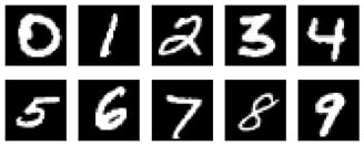
Figure 1.11 – MNIST digit examples
In this experiment, we simplify the problem by casting images into binary format with only two possible values: 0 represents black and 1 represents white. The code for this is as follows:
def binarize(image, label):
    image = tf.cast(image, tf.float32)
    image = tf.math.round(image/255.)
    return image, tf.cast(image, tf.int32)
The function expects two inputs – an image and a label. The first two lines of the function cast the image into binary float32 format, in other words 0.0 or 1.0. In this tutorial, we will not use the label information; instead, we cast the binary image into an integer and return it. We don't have to cast it to an integer, but let's just do it to stick to the convention of using an integer for labels. To recap, both the input and the label are binary MNIST images of 28 x 28 x 1; they differ only in data type.
Masking
Unlike PixelRNN, which reads row by row, PixelCNN slides a convolutional kernel across the image from left to right and from top to bottom. When performing convolution to predict the current pixel, a conventional convolution kernel is able to see the current input pixel together with the pixels surrounding it, including future pixels, and this breaks our conditional probability assumptions.
To avoid that, we need to make sure that the CNN doesn't cheat to look at the pixel it is predicting. In other words, we need to make sure that the CNN doesn't see the input pixel xi while it is predicting the output pixel xi.
This is by using a masked convolution, where a mask is applied to the convolutional kernel weights before performing convolution. The following diagram shows a mask for a 7 x 7 kernel, where the weight from the center onward is 0. This blocks the CNN from seeing the pixel it is predicting (the center of the kernel) and all future pixels. This is known as a type A mask and is applied only to the input layer. As the center pixel is blocked in the first layer, we don't need to hide the center feature anymore in later layers. In fact, we will need to set the kernel center to 1 to enable it to read the features from previous layers. This is known as type B Mask:

Figure 1.12 – A 7 x 7 kernel mask (Source: Aäron van den Oord et al., 2016, Conditional Image Generation with PixelCNN Decoders, https://arxiv.org/abs/1606.05328)
Next, we will learn how to create a custom layer.
Implementing a custom layer
We will now create a custom layer for the masked convolution. We can create a custom layer in TensorFlow using model subclassing inherited from the base class, tf.keras.layers.Layer, as shown in the following code. We will be able to use it just like other Keras layers. The following is the basic structure of the custom layer class:
class MaskedConv2D(tf.keras.layers.Layer):
    def __init__(self):
        ...
    def build(self, input_shape):
        ...
    def call(self, inputs):
        ...
        return output
build() takes the input tensor's shape as an argument, and we will use this information to create variables of the correct shapes. This function runs only once, when the layer is built. We can create a mask by declaring it either as a non-trainable variable or as a constant to let TensorFlow know it does not need to have gradients to backpropagate:
    def build(self, input_shape):
        self.w = self.add_weight(shape=[self.kernel,
                                        self.kernel,
                                        input_shape[-1],
                                        self.filters],
                                initializer='glorot_normal',
                                trainable=True)
        self.b = self.add_weight(shape=(self.filters,),
                                initializer='zeros',
                                trainable=True)
        mask = np.ones(self.kernel**2, dtype=np.float32)
        center = len(mask)//2
        mask[center+1:] = 0
        if self.mask_type == 'A':
            mask[center] = 0
        mask = mask.reshape((self.kernel, self.kernel, 1, 1))
        self.mask = tf.constant(mask, dtype='float32')
call() is the forward pass that performs the computation. In this masked convolutional layer, we multiply the weight by the mask to zero the lower half before performing convolution using the low-level tf.nn API:
    def call(self, inputs):
        masked_w = tf.math.multiply(self.w, self.mask)
        output = tf.nn.conv2d(inputs, masked_w, 1, "SAME") +  	                   self.b
        return output
Tips
tf.keras.layers is a high-level API that is easy to use without you needing to know under-the-hood details. However, sometimes we will need to create custom functions using the low-level tf.nn API, which requires us to first specify or create the tensors to be used.
Network layers
The PixelCNN architecture is quite straightforward. After the first 7 x 7 conv2d layer with mask A, there are several layers of residual blocks (see the following table) with mask B. To keep the same feature map size of 28 x 28, there is no downsampling; for example, the max pooling and padding in these layers is set to SAME. The top features are then fed into two layers of 1 x 1 convolution layers before the output is produced, as seen in the following screenshot:
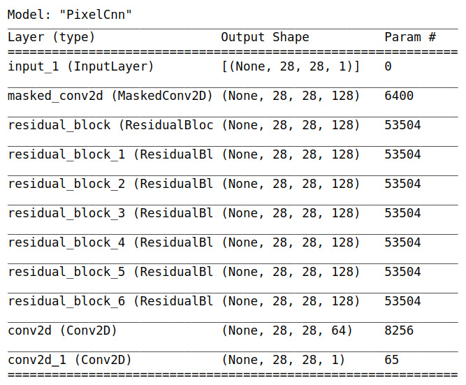
Figure 1.13 – The PixelCNN architecture, showing the layers and output shape
Residual blocks are used in many high-performance CNN-based models and were made popular by ResNet, which was invented by Kaiming He et al. in 2015. The following diagram illustrates a variant of residual blocks used in PixelCNN. The left path is called a skip connection path, which simply passes the features from the previous layer. On the right path are three sequential convolutional layers with filters of 1 x 1, 3 x 3, and 1 x 1. This path optimizes the residuals of the input features, hence the name residual net:
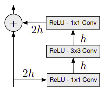
Figure 1.14 – The residual block where h is the number of filters. (Source: Aäron van den Oord et al., Pixel Recurrent Neural Networks)
Cross-entropy loss
Cross-entropy loss, also known as log loss, measures the performance of a model, where the output's probability is between 0 and 1. The following is the equation for binary cross-entropy loss, where there are only two classes, labels y can be either 0 or 1, and p(x) is the model's prediction. The equation is as follows:

Let's look at an example where the label is 1, the second term is zero, and the first term is the sum of log p(x). The log in the equation is natural log (loge) but by convention the base of e is omitted from the equations. If the model is confident that x belongs to label 1, then log(1) is zero. On the other hand, if the model wrongly guesses it as label 0 and predicts a low probability of x being label 1, say p(x) = 0.1. Then -log (p(x)) becomes higher loss of 2.3. Therefore, minimizing cross-entropy loss will maximize the model's accuracy. This loss function is commonly used in classification models but is also popular among generative models.
In PixelCNN, the individual image pixel is used as a label. In our binarized MNIST, we want to predict whether the output pixel is either 0 or 1, which makes this a classification problem with cross-entropy as the loss function.
There can be two output types:
- Since there can only be 0 or 1 in a binarized image, we can simplify the network by using
sigmoid()to predict the probability of a white pixel, that is, p(xi = 1). The loss function is binary cross-entropy. This is what we will use in our PixelCNN model. - Optionally, we could also generalize the network to accept grayscale or RGB images. We can use the
softmax()activation function to produce N probabilities for each (sub)pixel. N will be 2 for binarized images, 256 for grayscale images, and 3 x 256 for RGB images. The loss function is sparse categorical cross-entropy or categorical cross-entropy if the label is one-hot encoded.
Finally, we are now ready to compile and train the neural network. As seen in the following code, we use binary cross-entropy for both loss and metrics and use RMSprop as the optimizer. There are many different optimizers to use, and their main difference comes in how they adjust the learning rate of individual variables based on past statistics. Some optimizers accelerate training but may tend to overshoot and not achieve global minima. There is no one best optimizer to use in all cases, and you are encouraged to try different ones.
However, the two optimizers that you will see a lot are Adam and RMSprop. The Adam optimizer is a popular choice in image generation for its fast learning, while RMSprop is used frequently by Google to produce state-of-the-art models.
The following is used to compile and fit the pixelcnn model:
pixelcnn = SimplePixelCnn()
pixelcnn.compile(
    loss = tf.keras.losses.BinaryCrossentropy(),
    optimizer=tf.keras.optimizers.RMSprop(learning_rate=0.001),
    metrics=[ tf.keras.metrics.BinaryCrossentropy()])
pixelcnn.fit(ds_train, epochs = 10, validation_data=ds_test)
Next, we will generate a new image from the preceding model.
Sample image
After the training, we can generate a new image using the model by taking the following steps:
- Create an empty tensor with the same shape as the input image and fill it with zeros. Feed this into the network and get p(x1), the probability of the first pixel.
- Sample from p(x1) and assign the sample value to pixel x1 in the input tensor.
- Feed the input to the network again and perform step 2 for the next pixel.
- Repeat steps 2 and 3 until xN has been generated.
One major drawback of the autoregressive model is that it is slow because of the need to generate pixel by pixel, which cannot be parallelized. The following images were generated by our simple PixelCNN model after 50 epochs of training. They don't look quite like proper digits yet, but they're starting to take the shape of handwriting strokes. It's quite amazing that we can now generate new images out of thin air (that is, with zero-input tensors). Can you generate better digits by training the model longer and doing some hyperparameter tuning?

Figure 1.15 – Some images generated by our PixelCNN model
With that, we have come to the end of the chapter!


