Why causality? Ask babies!
Is there anything missing from Hume’s theory of causation? Although many other philosophers tried to answer this question, we’ll focus on one particularly interesting answer that comes from… human babies.
Interacting with the world
Alison Gopnik is an American child psychologist who studies how babies develop their world models. She also works with computer scientists, helping them understand how human babies build common-sense concepts about the external world. Children – to an even greater extent than adults – make use of associative learning, but they are also insatiable experimenters.
Have you ever seen a parent trying to convince their child to stop throwing around a toy? Some parents tend to interpret this type of behavior as rude, destructive, or aggressive, but babies often have a different set of motivations. They are running systematic experiments that allow them to learn the laws of physics and the rules of social interactions (Gopnik, 2009). Infants as young as 11 months prefer to perform experiments with objects that display unpredictable properties (for example, can pass through a wall) than with objects that behave predictably (Stahl & Feigenson, 2015). This preference allows them to efficiently build models of the world.
What we can learn from babies is that we’re not limited to observing the world, as Hume suggested. We can also interact with it. In the context of causal inference, these interactions are called interventions, and we’ll learn more about them in Chapter 2. Interventions are at the core of what many consider the Holy Grail of the scientific method: randomized controlled trial, or RCT for short.
Confounding – relationships that are not real
The fact that we can run experiments enhances our palette of possibilities beyond what Hume thought about. This is very powerful! Although experiments cannot solve all of the philosophical problems related to gaining new knowledge, they can solve some of them. A very important aspect of a properly designed randomized experiment is that it allows us to avoid confounding. Why is it important?
A confounding variable influences two or more other variables and produces a spurious association between them. From a purely statistical point of view, such associations are indistinguishable from the ones produced by a causal mechanism. Why is that problematic? Let’s see an example.
Imagine you work at a research institute and you’re trying to understand the causes of people drowning. Your organization provides you with a huge database of socioeconomic variables. You decide to run a regression model over a large set of these variables to predict the number of drownings per day in your area of interest. When you check the results, it turns out that the biggest coefficient you obtained is for daily regional ice cream sales. Interesting! Ice cream usually contains large amounts of sugar, so maybe sugar affects people’s attention or physical performance while they are in the water.
This hypothesis might make sense, but before we move forward, let’s ask some questions. How about other variables that we did not include in the model? Did we add enough predictors to the model to describe all relevant aspects of the problem? What if we added too many of them? Could adding just one variable to the model completely change the outcome?
Adding too many predictors
Adding too many predictors to the model might be harmful from both statistical and causal points of view. We will learn more on this topic in Chapter 3.
It turns out that this is possible.
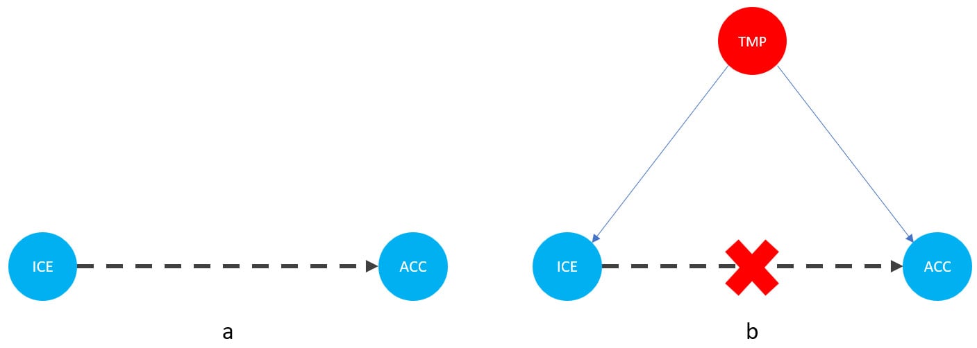
Let me introduce you to daily average temperature – our confounder. Higher daily temperature makes people more likely to buy ice cream and more likely to go swimming. When there are more people swimming, there are also more accidents. Let’s try to visualize this relationship:

Figure 1.1 – Graphical representation of models with two (a) and three variables (b). Dashed lines represent the association, solid lines represent causation. ICE = ice cream sales, ACC = the number of accidents, and TMP = temperature.
In Figure 1.1, we can see that adding the average daily temperature to the model removes the relationship between regional ice cream sales and daily drownings. Depending on your background, this might or might not be surprising to you. We’ll learn more about the mechanism behind this effect in Chapter 3.
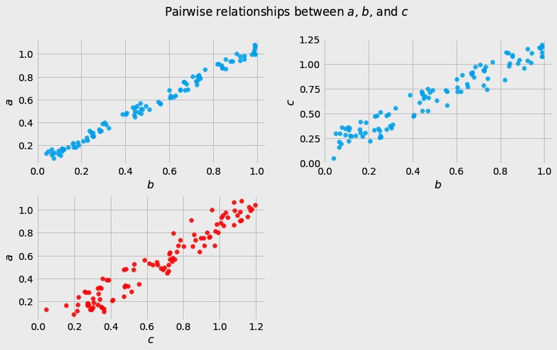
Before we move further, we need to state one important thing explicitly: confounding is a strictly causal concept. What does it mean? It means that we’re not able to say much about confounding using purely statistical language (note that this means that Hume’s definition as we presented it here cannot capture it). To see this clearly, let’s look at Figure 1.2:

Figure 1.2 – Pairwise scatterplots of relations between a, b, and c. The code to recreate the preceding plot can be found in the Chapter_01.ipynb notebook (https://github.com/PacktPublishing/Causal-Inference-and-Discovery-in-Python/blob/main/Chapter_01.ipynb).
In Figure 1.2, blue points signify a causal relationship while red points signify a spurious relationship, and variables a, b, and c are related in the following way:
- b causes a and c
- a and c are causally independent
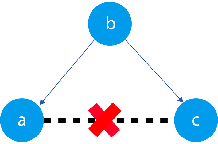
Figure 1.3 presents a graphical representation of these relationships:

Figure 1.3 – Relationships between a, b, and c
The black dashed line with the red cross denotes that there is no causal relationship between a and c in any direction.
Hey, but in Figure 1.2 we see some relationship! Let’s unpack it!
In Figure 1.2, non-spurious (blue) and spurious (red) relationships look pretty similar to each other and their correlation coefficients will be similarly large. In practice, most of the time, they just cannot be distinguished based on solely statistical criteria and we need causal knowledge to distinguish between them.
Asymmetries and causal discovery
If fact, in some cases, we can use noise distribution or functional asymmetries to find out which direction is causal. This information can be leveraged to recover causal structure from observational data, but it also requires some assumptions about the data-generating process. We’ll learn more about this in Part 3, Causal Discovery (Chapter 13).
Okay, we said that there are some spurious relationships in our data; we added another variable to the model and it changed the model’s outcome. That said, I was still able to make useful predictions without this variable. If that’s true, why would I care whether the relationship is spurious or non-spurious? Why would I care whether the relationship is causal or not?


