Search icon CANCEL
Subscription
0
Cart icon
Your Cart (0 item)
Close icon
You have no products in your basket yet
Save more on your purchases! discount-offer-chevron-icon
Savings automatically calculated. No voucher code required.
Arrow left icon
Explore Products
Best Sellers
New Releases
Books
Videos
Audiobooks
Learning Hub
Free Learning
Arrow right icon
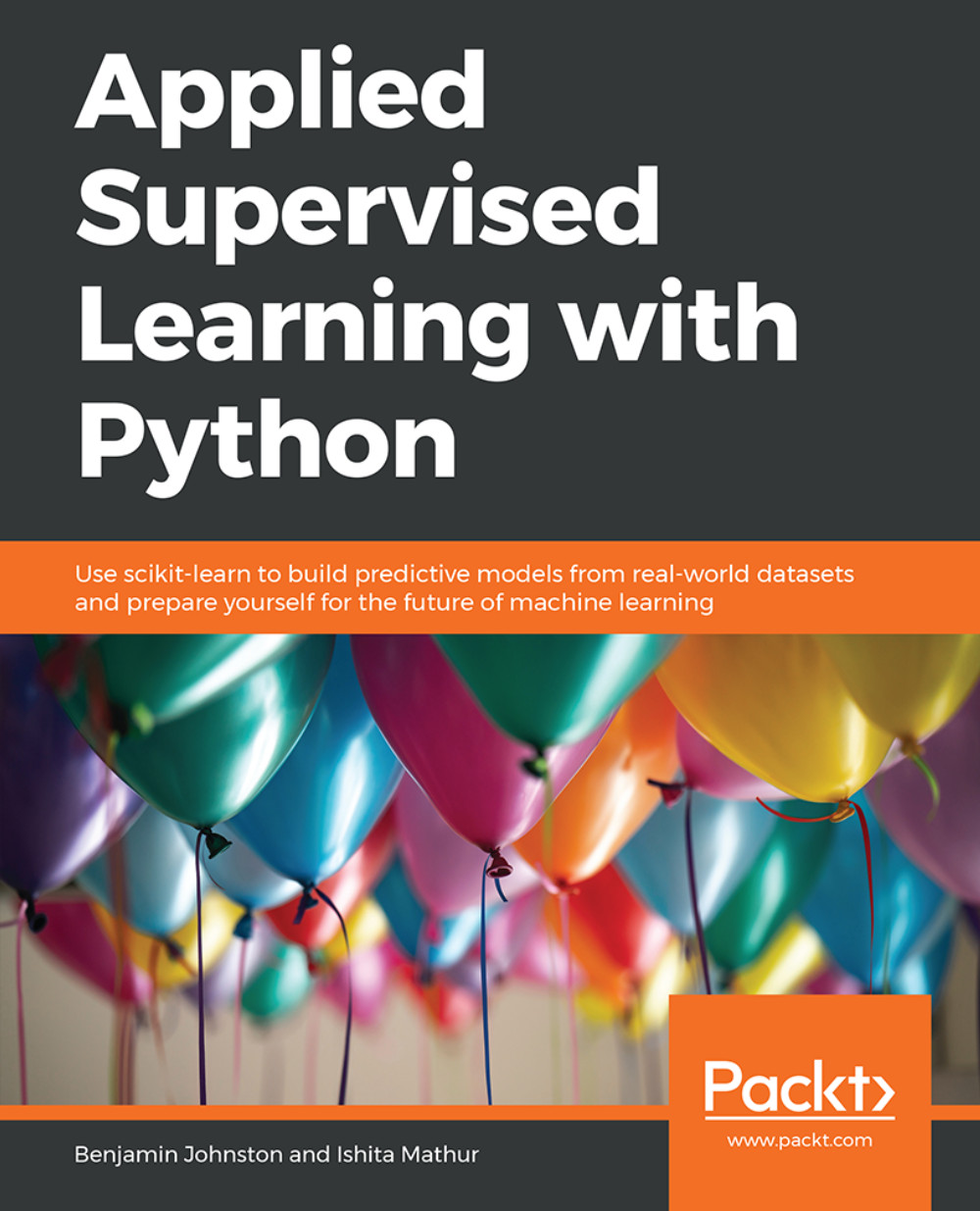
Applied Supervised Learning with Python

Applied Supervised Learning with Python: Use scikit-learn to build predictive models from real-world datasets and prepare yourself for the future of machine learning

Arrow left icon
Profile Icon Benjamin Johnston Profile Icon Mathur
Arrow right icon
£7.99 £26.99
Full star icon Full star icon Full star icon Full star icon Full star icon 5 (1 Ratings)
eBook Apr 2019 404 pages 1st Edition
eBook
£7.99 £26.99
Paperback
£32.99
Subscription
Free Trial
Renews at £16.99p/m
eBook
£7.99 £26.99
Paperback
£32.99
Subscription
Free Trial
Renews at £16.99p/m

What do you get with eBook?

Product feature icon Instant access to your Digital eBook purchase
Product feature icon Download this book in EPUB and PDF formats
Product feature icon Access this title in our online reader with advanced features
Product feature icon DRM FREE - Read whenever, wherever and however you want
Product feature icon AI Assistant (beta) to help accelerate your learning
OR
Modal Close icon
Payment Processing...
tick Completed

Billing Address

Table of content icon View table of contents Preview book icon Preview Book

Applied Supervised Learning with Python

Chapter 1. Python Machine Learning Toolkit

Note

Learning Objectives

By the end of this chapter, you will be able to:

  • Explain supervised machine learning and describe common examples of machine learning problems

  • Install and load Python libraries into your development environment for use in analysis and machine learning problems

  • Access and interpret the documentation of a subset of Python libraries, including the powerful pandas library

  • Create an IPython Jupyter notebook and use executable code cells and markdown cells to create a dynamic report

  • Load an external data source using pandas and use a variety of methods to search, filter, and compute descriptive statistics of the data

  • Clean a data source of mediocre quality and gauge the potential impact of various issues within the data source

Note

This chapter introduces supervised learning, Jupyter notebooks, and some of the most common pandas data methods.

Introduction


The study and application of machine learning and artificial intelligence has recently been the source of much interest and research in the technology and business communities. Advanced data analytics and machine learning techniques have shown great promise in advancing many sectors, such as personalized healthcare and self-driving cars, as well as in solving some of the world's greatest challenges, such as combating climate change. This book has been designed to assist you in taking advantage of the unique confluence of events in the field of data science and machine learning today. Across the globe, private enterprises and governments are realizing the value and efficiency of data-driven products and services. At the same time, reduced hardware costs and open source software solutions are significantly reducing the barriers to entry of learning and applying machine learning techniques.

Throughout this book, you will develop the skills required to identify, prepare, and build predictive models using supervised machine learning techniques in the Python programming language. The six chapters each cover one aspect of supervised learning. This chapter introduces a subset of the Python machine learning toolkit, as well as some of the things that need to be considered when loading and using data sources. This data exploration process is further explored in Chapter 2, Exploratory Data Analysis and Visualization, as we introduce exploratory data analysis and visualization. Chapter 3, Regression Analysis, and Chapter 4, Classification, look at two subsets of machine learning problems – regression and classification analysis – and demonstrate these techniques through examples. Finally, Chapter 5, Ensemble Modeling, covers ensemble networks, which use multiple predictions from different models to boost overall performance, while Chapter 6, Model Evaluation, covers the extremely important concepts of validation and evaluation metrics. These metrics provide a means of estimating the true performance of a model.

Supervised Machine Learning


A machine learning algorithm is commonly thought of as simply the mathematical process (or algorithm) itself, such as a neural network, deep neural network, or random forest algorithm. However, this is only a component of the overall system; firstly, we must define the problem that can be adequately solved using such techniques. Then, we must specify and procure a clean dataset that is composed of information that can be mapped from the first number space to a secondary one. Once the dataset has been designed and procured, the machine learning model can be specified and designed; for example, a single-layer neural network with 100 hidden nodes that uses a tanh activation function.

With the dataset and model well defined, the means of determining the exact values for the model can be specified. This is a repetitive optimization process that evaluates the output of the model against some existing data and is commonly referred to as training. Once training has been completed and you have your defined model, then it is good practice to evaluate it against some reference data to provide a benchmark of overall performance.

Considering this general description of a complete machine learning algorithm, the problem definition and data collection stages are often the most critical. What is the problem you are trying to solve? What outcome would you like to achieve? How are you going to achieve it? How you answer these questions will drive and define many of the subsequent decisions or model design choices. It is also in answering these questions that we will select which category of machine learning algorithms we will choose: supervised or unsupervised methods.

So, what exactly are supervised and unsupervised machine learning problems or methods? Supervised learning techniques center on mapping some set of information to another by providing the training process with the input information and the desired outputs, then checking its ability to provide the correct result. As an example, let's say you are the publisher of a magazine that reviews and ranks hairstyles from various time periods. Your readers frequently send you far more images of their favorite hairstyles for review than you can manually process. To save some time, you would like to automate the sorting of the hairstyles images you receive based on time periods, starting with hairstyles from the 1960s and 1980s:

Figure 1.1: Hairstyles images from different time periods

To create your hairstyles-sorting algorithm, you start by collecting a large sample of hairstyles images and manually labeling each one with its corresponding time period. Such a dataset (known as a labeled dataset) is the input data (hairstyles images) and the desired output information (time period) is known and recorded. This type of problem is a classic supervised learning problem; we are trying to develop an algorithm that takes a set of inputs and learns to return the answers that we have told it are correct.

When to Use Supervised Learning

Generally, if you are trying to automate or replicate an existing process, the problem is a supervised learning problem. Supervised learning techniques are both very useful and powerful, and you may have come across them or even helped create labeled datasets for them without realizing. As an example, a few years ago, Facebook introduced the ability to tag your friends in any image uploaded to the platform. To tag a friend, you would draw a square over your friend's face and then add the name of your friend to notify them of the image. Fast-forward to today and Facebook will automatically identify your friends in the image and tag them for you. This is yet another example of supervised learning. If you ever used the early tagging system and manually identified your friends in an image, you were in fact helping to create Facebook's labeled dataset. A user who uploaded an image of a person's face (the input data) and tagged the photo with the subject's name would then create the label for the dataset. As users continued to use this tagging service, a sufficiently large labeled dataset was created for the supervised learning problem. Now friend-tagging is completed automatically by Facebook, replacing the manual process with a supervised learning algorithm, as opposed to manual user input:

Figure 1.2: Tagging a friend on Facebook

One particularly timely and straightforward example of supervised learning is the training of self-driving cars. In this example, the algorithm uses the target route as determined by the GPS system, as well as on-board instrumentation, such as speed measures, the brake position, and/or a camera or Light Detection and Ranging (LIDAR), for road obstacle detection as the labeled outputs of the system. During training, the algorithm samples the control inputs as provided by the human driver, such as speed, steering angle, and brake position, mapping them against the outputs of the system; thus providing the labeled dataset. This data can then be used to train the driving/navigation systems within the self-driving car or in simulation exercises.

Image-based supervised problems, while popular, are not the only examples of supervised learning problems. Supervised learning is also commonly used in the automatic analysis of text to determine whether the opinion or tone of a message is positive, negative, or neutral. Such analysis is known as sentiment analysis and frequently involves creating and using a labeled dataset of a series of words or statements that are manually identified as either positive, neutral, or negative. Consider these sentences: I like that movie and I hate that movie. The first sentence is clearly positive, while the second is negative. We can then decompose the words in the sentences into either positive, negative, or neutral (both positive, both negative); see the following table:


Figure 1.3: Decomposition of the words

Using sentiment analysis, a supervised learning algorithm could be created, say, using the movie database site IMDb to analyze comments posted about movies to determine whether the movie is being positively or negatively reviewed by the audience. Supervised learning methods could have other applications, such as analyzing customer complaints, automating troubleshooting calls/chat sessions, or even medical applications such as analyzing images of moles to detect abnormalities (https://www.nature.com/articles/nature21056).

This should give you a good understanding of the concept of supervised learning, as well as some examples of problems that can be solved using these techniques. While supervised learning involves training an algorithm to map the input information to corresponding known outputs, unsupervised learning methods, by contrast, do not utilize known outputs, either because they are not available or even known. Rather than relying on a set of manually annotated labels, unsupervised learning methods model the supplied data through specific constraints or rules designed into the training process.

Clustering analysis is a common form of unsupervised learning where a dataset is to be divided into a specified number of different groups based on the clustering process being used. In the case of k-nearest neighbors clustering, each sample from the dataset is labeled or classified in accordance with the majority vote of the k-closest points to the sample. As there are no manually identified labels, the performance of unsupervised algorithms can vary greatly with the data being used, as well as the selected parameters of the model. For example, should we use the 5 closest or 10 closest points in the majority vote of the k-closest points? The lack of known and target outputs during training leads to unsupervised methods being commonly used in exploratory analysis or in scenarios where the ground truth targets are somewhat ambiguous and are better defined by the constraints of the learning method.

We will not cover unsupervised learning in great detail in this book, but it is useful to summarize the main difference between the two methods. Supervised learning methods require ground truth labels or the answers for the input data, while unsupervised methods do not use such labels, and the final result is determined by the constraints applied during the training process.

Why Python?

So, why have we chosen the Python programming language for our investigation into supervised machine learning? There are a number of alternative languages available, including C++, R, and Julia. Even the Rust community is developing machine learning libraries for their up-and-coming language. There are a number of reasons why Python is the first-choice language for machine learning:

  • There is great demand for developers with Python expertise in both industry and academic research.

  • Python is currently one of the most popular programming languages, even reaching the number one spot in IEEE Spectrum magazine's survey of the top 10 programming languages (https://spectrum.ieee.org/at-work/innovation/the-2018-top-programming-languages).

  • Python is an open source project, with the entire source code for the Python programming language being freely available under the GNU GPL Version 2 license. This licensing mechanism has allowed Python to be used, modified, and even extended in a number of other projects, including the Linux operating system, supporting NASA (https://www.python.org/about/success/usa/), and a plethora of other libraries and projects that have provided additional functionality, choice, and flexibility to the Python programming language. In our opinion, this flexibility is one of the key components that has made Python so popular.

  • Python provides a common set of features that can be used to run a web server, a microservice on an embedded device, or to leverage the power of graphical processing units to perform precise calculations on large datasets.

  • Using Python and a handful of specific libraries (or packages, as they are known in Python), an entire machine learning product can be developed—starting with exploratory data analysis, model definition, and refinement, through to API construction and deployment. All of these steps can be completed within Python to build an end-to-end solution. This is the significant advantage Python has over some of its competitors, particularly within the data science and machine learning space. While R and Julia have the advantage of being specifically designed for numerical and statistical computing, models developed in these languages typically require translation into some other language before they can be deployed in a production setting.

We hope that, through this book, you will gain an understanding of the flexibility and power of the Python programming language and will start on the path of developing end-to-end supervised learning solutions in Python. So, let's get started.

Jupyter Notebooks


One aspect of the data science development environment that distinguishes itself from other Python projects is the use of IPython Jupyter notebooks (https://jupyter.org). Jupyter notebooks provide a means of creating and sharing interactive documents with live, executable code snippets, and plots, as well as the rendering of mathematical equations through the Latex (https://www.latex-project.org) typesetting system. This section of the chapter will introduce you to Jupyter notebooks and some of their key features to ensure your development environment is correctly set up.

Throughout this book, we will make frequent reference to the documentation for each of the introduced tools/packages. The ability to effectively read and understand the documentation for each tool is extremely important. Many of the packages we will use contain so many features and implementation details that it is very difficult to memorize them all. The following documentation may come in handy for the upcoming section on Jupyter notebooks:

  • The Anaconda documentation can be found at https://docs.anaconda.com.

  • The Anaconda user guide can be found at https://docs.anaconda.com/anaconda/user-guide.

  • The Jupyter Notebook documentation can be found at https://jupyter-notebook.readthedocs.io/en/stable/.

Exercise 1: Launching a Jupyter Notebook

In this exercise, we will launch our Jupyter notebook. Ensure you have correctly installed Anaconda with Python 3.7, as per the Preface:

  1. There are two ways of launching a Jupyter notebook through Anaconda. The first method is to open Jupyter using the Anaconda Navigator application available in the Anaconda folder of the Windows Start menu. Click on the Launch button and your default internet browser will then launch at the default address, http://localhost:8888, and will start in a default folder path.

  2. The second method is to launch Jupyter via the Anaconda prompt. To launch the Anaconda prompt, simply click on the Anaconda Prompt menu item, also in the Windows Start menu, and you should see a pop-up window similar to the following screenshot:

    Figure 1.4: Anaconda prompt

  3. Once in the Anaconda prompt, change to the desired directory using the cd (change directory) command. For example, to change into the Desktop directory for the Packt user, do the following:

    C:\Users\Packt> cd C:\Users\Packt\Desktop
  4. Once in the desired directory, launch a Jupyter notebook using the following command:

    C:\Users\Packt> jupyter notebook

    The notebook will launch with the working directory from the one you specified earlier. This then allows you to navigate and save your notebooks in the directory of your choice as opposed to the default, which can vary between systems, but is typically your home or My Computer directory. Irrespective of the method of launching Jupyter, a window similar to the following will open in your default browser. If there are existing files in the directory, you should also see them here:

    Figure 1.5: Jupyter notebook launch window

Exercise 2: Hello World

The Hello World exercise is a rite of passage, so you certainly cannot be denied that experience! So, let's print Hello World in a Jupyter notebook in this exercise:

  1. Start by creating a new Jupyter notebook by clicking on the New button and selecting Python 3. Jupyter allows you to run different versions of Python and other languages, such as R and Julia, all in the same interface. We can also create new folders or text files here too. But for now, we will start with a Python 3 notebook:

    Figure 1.6: Creating a new notebook

    This will launch a new Jupyter notebook in a new browser window. We will first spend some time looking over the various tools that are available in the notebook:

    Figure 1.7: The new notebook

    There are three main sections in each Jupyter notebook, as shown in the following screenshot: the title bar (1), the toolbar (2), and the body of the document (3). Let's look at each of these components in order:

    Figure 1.8: Components of the notebook

  2. The title bar simply displays the name of the current Jupyter notebook and allows the notebook to be renamed. Click on the Untitled text and a popup will appear allowing you to rename the notebook. Enter Hello World and click Rename:

    Figure 1.9: Renaming the notebook

  3. For the most part, the toolbar contains all the normal functionality that you would expect. You can open, save, and make copies of—or create new—Jupyter notebooks in the File menu. You can search replace, copy, and cut content in the Edit menu and adjust the view of the document in the View menu. As we discuss the body of the document, we will also describe some of the other functionalities in more detail, such as the ones included in the Insert, Cell, and Kernel menus. One aspect of the toolbar that requires further examination is the far right-hand side, the outline of the circle on the right of Python 3.

    Hover your mouse over the circle and you will see the Kernel Idle popup. This circle is an indicator to signify whether the Python kernel is currently processing; when processing, this circle indicator will be filled in. If you ever suspect that something is running or is not running, you can easily refer to this icon for more information. When the Python kernel is not running, you will see this:

    Figure 1.10: Kernel idle

    When the Python kernel is running, you will see this:

    Figure 1.11: Kernel busy

  4. This brings us to the body of the document, where the actual content of the notebook will be entered. Jupyter notebooks differ from standard Python scripts or modules, in that they are divided into separate executable cells. While Python scripts or modules will run the entirety of the script when executed, Jupyter notebooks can run all of the cells sequentially, or can also run them separately and in a different order if manually executed.

    Double-click on the first cell and enter the following:

    >>> print('Hello World!')
  5. Click on Run (or use the Ctrl + Enter keyboard shortcut):

    Figure 1.12: Running a cell

Congratulations! You just completed Hello World in a Jupyter notebook.

Exercise 3: Order of Execution in a Jupyter Notebook

In the previous exercise, notice how the print statement is executed under the cell. Now let's take it a little further. As mentioned earlier, Jupyter notebooks are composed of a number of separately executable cells; it is best to think of them as just blocks of code you have entered into the Python interpreter, and the code is not executed until you press the Ctrl + Enter keys. While the code is run at a different time, all of the variables and objects remain in the session within the Python kernel. Let's investigate this a little further:

  1. Launch a new Jupyter notebook and then, in three separate cells, enter the code shown in the following screenshot:

    Figure 1.13: Entering code into multiple cells

  2. Click Restart & Run All.

    Notice that there are three executable cells, and the order of execution is shown in rectangular brackets; for example, In [1], In [2], and In [3]. Also note how the hello_world variable is declared (and thus executed) in the second cell and remains in memory, and thus is printed in the third cell. As we mentioned before, you can also run the cells out of order.

  3. Click on the second cell, containing the declaration of hello_world, change the value to add a few more exclamation points, and run the cell again:

    Figure 1.14: Changing the content of the second cell

    Notice that the second cell is now the most recently executed cell (In [4]), and that the print statement after it has not been updated. To update the print statement, you would then need to execute the cell below it. Warning: be careful about your order of execution. If you are not careful, you can easily override values or declare variables in cells below their first use, as in notebooks, you no longer need to run the entire script at once. As such, it is good practice to regularly click Kernel | Restart & Run All. This will clear all variables from memory and run all cells from top to bottom in order. There is also the option to run all cells below or above a particular cell in the Cell menu:

    Figure 1.15: Restarting the kernel

    Note

    Write and structure your notebook cells as if you were to run them all in order, top to bottom. Use manual cell execution only for debugging/early investigation.

  4. You can also move cells around using either the up/down arrows on the left of Run or through the Edit toolbar. Move the cell that prints the hello_world variable to above its declaration:

    Figure 1.16: Moving cells

  5. Click on Restart & Run All cells:

    Figure 1.17: Variable not defined error

    Notice the error reporting that the variable is not defined. This is because it is being used before its declaration. Also, notice that the cell after the error has not been executed as shown by the empty In [ ].

Exercise 4: Advantages of Jupyter Notebooks

There are a number of additional features of Jupyter notebooks that make them very useful. In this exercise, we will examine some of these features:

  1. Jupyter notebooks can execute commands directly within the Anaconda prompt by including an exclamation point prefix (!). Enter the code shown in the following screenshot and run the cell:

    Figure 1.18: Running Anaconda commands

  2. One of the best features of Jupyter notebooks is the ability to create live reports that contain executable code. Not only does this save time in preventing separate creation of reports and code, but it can also assist in communicating the exact nature of the analysis being completed. Through the use of Markdown and HTML, we can embed headings, sections, images, or even JavaScript for dynamic content.

    To use Markdown in our notebook, we first need to change the cell type. First, click on the cell you want to change to Markdown, then click on the Code drop-down menu and select Markdown:

    Figure 1.19: Running Anaconda commands

    Notice that In [ ] has disappeared and the color of the box lining the cell is no longer blue.

  3. You can now enter valid Markdown syntax and HTML by double-clicking in the cell and then clicking Run to render the markdown. Enter the syntax shown in the following screenshot and run the cell to see the output:

    Figure 1.20: Markdown syntax

    The output will be as follows:

    Figure 1.21: Markdown output

    Note

    For a quick reference on Markdown, refer to the Markdown Syntax.ipynb Jupyter notebook in the code files for this chapter.

Python Packages and Modules

While the standard features that are included in Python are certainly feature-rich, the true power of Python lies in the additional libraries (also known as packages in Python), which, thanks to open source licensing, can be easily downloaded and installed through a few simple commands. In an Anaconda installation, it is even easier as many of the most common packages come pre-built within Anaconda. You can get a complete list of the pre-installed packages in the Anaconda environment by running the following command in a notebook cell:

!conda list

In this book, we will be using the following additional Python packages:

  • NumPy (pronounced Num Pie and available at https://www.numpy.org/): NumPy (short for numerical Python) is one of the core components of scientific computing in Python. NumPy provides the foundational data types from which a number of other data structures derive, including linear algebra, vectors and matrices, and key random number functionality.

  • SciPy (pronounced Sigh Pie and available at https://www.scipy.org): SciPy, along with NumPy, is a core scientific computing package. SciPy provides a number of statistical tools, signal processing tools, and other functionality, such as Fourier transforms.

  • pandas (available at https://pandas.pydata.org/): pandas is a high-performance library for loading, cleaning, analyzing, and manipulating data structures.

  • Matplotlib (available at https://matplotlib.org/): Matplotlib is the foundational Python library for creating graphs and plots of datasets and is also the base package from which other Python plotting libraries derive. The Matplotlib API has been designed in alignment with the Matlab plotting library to facilitate an easy transition to Python.

  • Seaborn (available at https://seaborn.pydata.org/): Seaborn is a plotting library built on top of Matplotlib, providing attractive color and line styles as well as a number of common plotting templates.

  • Scikit-learn (available at https://scikit-learn.org/stable/): Scikit-learn is a Python machine learning library that provides a number of data mining, modeling, and analysis techniques in a simple API. Scikit-learn includes a number of machine learning algorithms out of the box, including classification, regression, and clustering techniques.

These packages form the foundation of a versatile machine learning development environment with each package contributing a key set of functionalities. As discussed, by using Anaconda, you will already have all of the required packages installed and ready for use. If you require a package that is not included in the Anaconda installation, it can be installed by simply entering and executing the following in a Jupyter notebook cell:

!conda install <package name>

As an example, if we wanted to install Seaborn, we'd run this:

!conda install seaborn

To use one of these packages in a notebook, all we need to do is import it:

import matplotlib

pandas


As mentioned before, pandas is a library for loading, cleaning, and analyzing a variety of different data structures. It is the flexibility of pandas, in addition to the sheer number of built-in features, that makes it such a powerful, popular, and useful Python package. It is also a great package to start with as, obviously, we cannot analyze any data if we do not first load it into the system. As pandas provides so much functionality, one very important skill in using the package is the ability to read and understand the documentation. Even after years of experience programming in Python and using pandas, we still refer to the documentation very frequently. The functionality within the API is so extensive that it is impossible to memorize all of the features and specifics of the implementation.

Note

The pandas documentation can be found at https://pandas.pydata.org/pandas-docs/stable/index.html.

Loading Data in pandas

pandas has the ability to read and write a number of different file formats and data structures, including CSV, JSON, and HDF5 files, as well as SQL and Python Pickle formats. The pandas input/output documentation can be found at https://pandas.pydata.org/pandas-docs/stable/user_guide/io.html. We will continue to look into the pandas functionality through loading data via a CSV file. The dataset we will be using for this chapter is the Titanic: Machine Learning from Disaster dataset, available from https://www.kaggle.com/c/Titanic/data or https://github.com/TrainingByPackt/Applied-Supervised-Learning-with-Python, which contains a roll of the guests on board the Titanic as well as their age, survival status, and number of siblings/parents. Before we get started with loading the data into Python, it is critical that we spend some time looking over the information provided for the dataset so that we can have a thorough understanding of what it contains. Download the dataset and place it in the directory you're working in.

Looking at the description for the data, we can see that we have the following fields available:

Figure 1.22: Fields in the Titanic dataset

We are also provided with some additional contextual information:

  • pclass: This is a proxy for socio-economic status, where first class is upper, second class is middle, and third class is lower status.

  • age: This is a fractional value if less than 1; for example, 0.25 is 3 months. If the age is estimated, it is in the form of xx.5.

  • sibsp: A sibling is defined as a brother, sister, stepbrother, or stepsister, and a spouse is a husband or wife.

  • parch: A parent is a mother or father, a child is a daughter, son, stepdaughter, or stepson. Children that traveled only with a nanny did not travel with a parent. Thus, 0 was assigned for this field.

  • embarked: The point of embarkation is the location where the passenger boarded the ship.

Note that the information provided with the dataset does not give any context as to how the data was collected. The survival, pclass, and embarked fields are known as categorical variables as they are assigned to one of a fixed number of labels or categories to indicate some other information. For example, in embarked, the C label indicates that the passenger boarded the ship at Cherbourg, and the value of 1 in survival indicates they survived the sinking.

Exercise 5: Loading and Summarizing the Titanic Dataset

In this exercise, we will read our Titanic dataset into Python and perform a few basic summary operations on it:

  1. Import the pandas package using shorthand notation, as shown in the following screenshot:

    Figure 1.23: Importing the pandas package

  2. Open the titanic.csv file by clicking on it in the Jupyter notebook home page:

    Figure 1.24: Opening the CSV file

    The file is a CSV file, which can be thought of as a table, where each line is a row in the table and each comma separates columns in the table. Thankfully, we don't need to work with these tables in raw text form and can load them using pandas:

    Figure 1.25: Contents of the CSV file

    Note

    Take a moment to look up the pandas documentation for the read_csv function at https://pandas.pydata.org/pandas-docs/stable/reference/api/pandas.read_csv.html. Note the number of different options available for loading CSV data into a pandas DataFrame.

  3. In an executable Jupyter notebook cell, execute the following code to load the data from the file:

    df = pd.read_csv('Titanic.csv')

    The pandas DataFrame class provides a comprehensive set of attributes and methods that can be executed on its own contents, ranging from sorting, filtering, and grouping methods to descriptive statistics, as well as plotting and conversion.

    Note

    Open and read the documentation for pandas DataFrame objects at https://pandas.pydata.org/pandas-docs/stable/reference/frame.html.

  4. Read the first five rows of data using the head() method of the DataFrame:

    df.head()

    Figure 1.26: Reading the first five rows

    In this sample, we have a visual representation of the information in the DataFrame. We can see that the data is organized in a tabular, almost spreadsheet-like structure. The different types of data are organized by columns, while each sample is organized by rows. Each row is assigned to an index value and is shown as the numbers 0 to 4 in bold on the left-hand side of the DataFrame. Each column is assigned to a label or name, as shown in bold at the top of the DataFrame.

The idea of a DataFrame as a kind of spreadsheet is a reasonable analogy; as we will see in this chapter, we can sort, filter, and perform computations on the data just as you would in a spreadsheet program. While not covered in this chapter, it is interesting to note that DataFrames also contain pivot table functionality, just like a spreadsheet (https://pandas.pydata.org/pandas-docs/stable/reference/api/pandas.pivot_table.html).

Exercise 6: Indexing and Selecting Data

Now that we have loaded some data, let's use the selection and indexing methods of the DataFrame to access some data of interest:

  1. Select individual columns in a similar way to a regular dictionary, by using the labels of the columns, as shown here:

    df['Age']

    Figure 1.27: Selecting the Age column

    If there are no spaces in the column name, we can also use the dot operator. If there are spaces in the column names, we will need to use the bracket notation:

    df.Age

    Figure 1.28: Using the dot operator to select the Age column

  2. Select multiple columns at once using bracket notation, as shown here:

    df[['Name', 'Parch', 'Sex']]

    Figure 1.29: Selecting multiple columns

  3. Select the first row using iloc:

    df.iloc[0]

    Figure 1.30: Selecting the first row

  4. Select the first three rows using iloc:

    df.iloc[[0,1,2]]

    Figure 1.31: Selecting the first three rows

  5. We can also get a list of all of the available columns. Do this as shown here:

    columns = df.columns # Extract the list of columns
    print(columns)

    Figure 1.32: Getting all the columns

  6. Use this list of columns and the standard Python slicing syntax to get columns 2, 3, and 4, and their corresponding values:

    df[columns[1:4]] # Columns 2, 3, 4

    Figure 1.33: Getting the second, third, and fourth columns

  7. Use the len operator to get the number of rows in the DataFrame:

    len(df)

    Figure 1.34: Getting the number of rows

  8. What if we wanted the value for the Fare column at row 2? There are a few different ways to do so. First, we'll try the row-centric methods. Do this as follows:

    df.iloc[2]['Fare'] # Row centric

    Figure 1.35: Getting a particular value using the normal row-centric method

  9. Try using the dot operator for the column. Do this as follows:

    df.iloc[2].Fare # Row centric

    Figure 1.36: Getting a particular value using the row-centric dot operator

  10. Try using the column-centric method. Do this as follows:

    df['Fare'][2] # Column centric

    Figure 1.37: Getting a particular value using the normal column-centric method

  11. Try the column-centric method with the dot operator. Do this as follows:

    df.Fare[2] # Column centric

    Figure 1.38: Getting a particular value using the column-centric dot operator

Exercise 7: Advanced Indexing and Selection

With the basics of indexing and selection under our belt, we can turn our attention to more advanced indexing and selection. In this exercise, we will look at a few important methods for performing advanced indexing and selecting data:

  1. Create a list of the passengers' names and ages for those passengers under the age of 21, as shown here:

    child_passengers = df[df.Age  < 21][['Name', 'Age']]
    child_passengers.head()

    Figure 1.39: List of the passengers' names and ages for those passengers under the age of 21

  2. Count how many child passengers there were, as shown here:

    print(len(child_passengers))

    Figure 1.40: Count of child passengers

  3. Count how many passengers were between the ages of 21 and 30. Do not use Python's and logical operator for this step, but rather the ampersand symbol (&). Do this as follows:

    young_adult_passengers = df.loc[
        (df.Age > 21) & (df.Age < 30)
    ]
    len(young_adult_passengers)

    Figure 1.41: Count of passengers between the ages of 21 and 30

  4. Count the passengers that were either first- or third-class ticket holders. Again, we will not use the Python logical or operator but rather the pipe symbol (|). Do this as follows:

    df.loc[
        (df.Pclass == 3) | (df.Pclass ==1)
    ]

    Figure 1.42: Count of passengers that were either first- or third-class ticket holders

  5. Count the passengers who were not holders of either first- or third-class tickets. Do not simply select the second class ticket holders, but rather use the ~ symbol for the not logical operator. Do this as follows:

    df.loc[
        ~((df.Pclass == 3) | (df.Pclass ==1))
    ]

    Figure 1.43: Count of passengers who were not holders of either first- or third-class tickets

  6. We no longer need the Unnamed: 0 column, so delete it using the del operator:

    del df['Unnamed: 0']
    df.head()

    Figure 1.44: The del operator

pandas Methods

Now that we are confident with some pandas basics, as well as some more advanced indexing and selecting tools, let's look at some other DataFrame methods. For a complete list of all methods available in a DataFrame, we can refer to the class documentation.

Note

The pandas documentation is available at https://pandas.pydata.org/pandas-docs/stable/reference/frame.html.

You should now know how many methods are available within a DataFrame. There are far too many to cover in detail in this chapter, so we will select a few that will give you a great start in supervised machine learning.

We have already seen the use of one method, head(), which provides the first five lines of the DataFrame. We can select more or less lines if we wish, by providing the number of lines as an argument, as shown here:

df.head(n=20) # 20 lines
df.head(n=32) # 32 lines

Another useful method is describe, which is a super-quick way of getting the descriptive statistics of the data within a DataFrame. We can see next that the sample size (count), mean, minimum, maximum, standard deviation, and 25th, 50th, and 75th percentiles are returned for all columns of numerical data in the DataFrame (note that text columns have been omitted):

df.describe()

Figure 1.45: The describe method

Note that only columns of numerical data have been included within the summary. This simple command provides us with a lot of useful information; looking at the values for count (which counts the number of valid samples), we can see that there are 1,046 valid samples in the Age category, but 1,308 in Fare, and only 891 in Survived. We can see that the youngest person was 0.17 years, the average age is 29.898, and the eldest 80. The minimum fare was £0, with £33.30 the average and £512.33 the most expensive. If we look at the Survived column, we have 891 valid samples, with a mean of 0.38, which means about 38% survived.

We can also get these values separately for each of the columns by calling the respective methods of the DataFrame, as shown here:

df.count()

Figure 1.46: The count method

But we have some columns that contain text data, such as Embarked, Ticket, Name, and Sex. So, what about these? How can we get some descriptive information for these columns? We can still use describe; we just need to pass it some more information. By default, describe will only include numerical columns and will compute the 25th, 50th, and 75th percentiles. But we can configure this to include text-based columns by passing the include = 'all' argument, as shown here:

df.describe(include='all')

Figure 1.47: The describe method with text-based columns

That's better—now we have much more information. Looking at the Cabin column, we can see that there are 295 entries, with 186 unique values. The most common values are C32, C25, and C27, and they occur 6 times (from the freq value). Similarly, if we look at the Embarked column, we see that there are 1,307 entries, 3 unique values, and that the most commonly occurring value is S with 914 entries.

Notice the occurrence of NaN values in our describe output table. NaN, or Not a Number, values are very important within DataFrames, as they represent missing or not available data. The ability of the pandas library to read from data sources that contain missing or incomplete information is both a blessing and a curse. Many other libraries would simply fail to import or read the data file in the event of missing information, while the fact that it can be read also means that the missing data must be handled appropriately.

When looking at the output of the describe method, you should notice that the Jupyter notebook renders it in the same way as the original DataFrame that we read in using read_csv. There is a very good reason for this, as the results returned by the describe method are themselves a pandas DataFrame and thus possess the same methods and characteristics as the data read in from the CSV file. This can be easily verified using Python's built-in type function:

Figure 1.48: Checking the type

Now that we have a summary of the dataset, let's dive in with a little more detail to get a better understanding of the available data.

Note

A comprehensive understanding of the available data is critical in any supervised learning problem. The source and type of the data, the means by which it is collected, and any errors potentially resulting from the collection process all have an effect on the performance of the final model.

Hopefully, by now, you are comfortable with using pandas to provide a high-level overview of the data. We will now spend some time looking into the data in greater detail.

Exercise 8: Splitting, Applying, and Combining Data Sources

We have already seen how we can index or select rows or columns from a DataFrame and use advanced indexing techniques to filter the available data based on specific criteria. Another handy method that allows for such selection is the groupby method, which provides a quick method for selecting groups of data at a time and provides additional functionality through the DataFrameGroupBy object:

  1. Use the groupby method to group the data by the Embarked column. How many different values for Embarked are there? Let's see:

    embarked_grouped = df.groupby('Embarked')
    
    print(f'There are {len(embarked_grouped)} Embarked groups')

    Figure 1.49: Grouping the data by the Embarked column

  2. What does the groupby method actually do? Let's check. Display the output of embarked_grouped.groups:

    embarked_grouped.groups

    Figure 1.50: Output of embarked_grouped.groups

    We can see here that the three groups are C, Q, and S, and that embarked_grouped.groups is actually a dictionary where the keys are the groups. The values are the rows or indexes of the entries that belong to that group.

  3. Use the iloc method to inspect row 1 and confirm that it belongs to embarked group C:

    df.iloc[1]

    Figure 1.51: Inspecting row 1

  4. As the groups are a dictionary, we can iterate through them and execute computations on the individual groups. Compute the mean age for each group, as shown here:

    for name, group in embarked_grouped:
        print(name, group.Age.mean())

    Figure 1.52: Computing the mean age for each group using iteration

  5. Another option is to use the aggregate method, or agg for short, and provide it the function to apply across the columns. Use the agg method to determine the mean of each group:

    embarked_grouped.agg(np.mean)

    Figure 1.53: Using the agg method

    So, how exactly does agg work and what type of functions can we pass it? Before we can answer these questions, we need to first consider the data type of each column in the DataFrame, as each column is passed through this function to produce the result we see here. Each DataFrame is comprised of a collection of columns of pandas series data, which in many ways operates just like a list. As such, any function that can take a list or a similar iterable and compute a single value as a result can be used with agg.

  6. As an example, define a simple function that returns the first value in the column, then pass that function through to agg:

    def first_val(x):
            
        return x.values[0]
    
    embarked_grouped.agg(first_val)

    Figure 1.54: Using the agg method with a function

Lambda Functions

One common and useful way of implementing agg is through the use of Lambda functions.

Lambda or anonymous functions (also known as inline functions in other languages) are small, single-expression functions that can be declared and used without the need for a formal function definition via use of the def keyword. Lambda functions are essentially provided for convenience and aren't intended to be used for extensive periods. The standard syntax for a Lambda function is as follows (always starting with the lambda keyword):

lambda <input values>: <computation for values to be returned>

Exercise 9: Lambda Functions

In this exercise, we will create a Lambda function that returns the first value in a column and use it with agg:

  1. Write the first_val function as a Lambda function, passed to agg:

    embarked_grouped.agg(lambda x: x.values[0])

    Figure 1.55: Using the agg method with a Lambda function

    Obviously, we get the same result, but notice how much more convenient the Lambda function was to use, especially given the fact that it is only intended to be used briefly.

  2. We can also pass multiple functions to agg via a list to apply the functions across the dataset. Pass the Lambda function as well as the NumPy mean and standard deviation functions, like this:

    embarked_grouped.agg([lambda x: x.values[0], np.mean, np.std])

    Figure 1.56: Using the agg method with multiple Lambda functions

  3. What if we wanted to apply different functions to different columns in the DataFrame? Apply numpy.sum to the Fare column and the Lambda function to the Age column by passing agg a dictionary where the keys are the columns to apply the function to and the values are the functions themselves:

    embarked_grouped.agg({
        'Fare': np.sum,
        'Age': lambda x: x.values[0]
    })

    Figure 1.57: Using the agg method with a dictionary of different columns

  4. Finally, you can also execute the groupby method using more than one column. Provide the method with a list of the columns (Sex and Embarked) to groupby, like this:

    age_embarked_grouped = df.groupby(['Sex', 'Embarked'])
    age_embarked_grouped.groups

    Figure 1.58: Using the groupby method with more than one column

    Similar to when the groupings were computed by just the Embarked column, we can see here that a dictionary is returned where the keys are the combination of the Sex and Embarked columns returned as a tuple. The first key-value pair in the dictionary is a tuple, ('Male', 'S'), and the values correspond to the indices of rows with that specific combination. There will be a key-value pair for each combination of unique values in the Sex and Embarked columns.

Data Quality Considerations


The quality of data used in any machine learning problem, supervised or unsupervised, is critical to the performance of the final model, and should be at the forefront when planning any machine learning project. As a simple rule of thumb, if you have clean data, in sufficient quantity, with a good correlation between the input data type and the desired output, then the specifics regarding the type and details of the selected supervised learning model become significantly less important to achieve a good result.

In reality, however, this can rarely be the case. There are usually some issues regarding the quantity of available data, the quality or signal-to-noise ratio in the data, the correlation between the input and output, or some combination of all three factors. As such, we will use this last section of this chapter to consider some of the data quality problems that may occur and some mechanisms for addressing them. Previously, we mentioned that in any machine learning problem, having a thorough understanding of the dataset is critical if we to are construct a high-performing model. This is particularly the case when looking into data quality and attempting to address some of the issues present within the data. Without a comprehensive understanding of the dataset, additional noise or other unintended issues may be introduced during the data cleaning process leading to a further degradation of performance.

Note

A detailed description of the Titanic dataset and the type of data included is contained in the Loading Data in pandas section. If you need a quick refresher, go back and review these details now.

Managing Missing Data

As we discussed earlier, the ability of pandas to read data with missing values is both a blessing and a curse and arguably is the most common issue that needs to be managed before we can continue with developing our supervised learning model. The simplest, but not necessarily the most effective, method is to just remove or ignore those entries that are missing data. We can easily do this in pandas using the dropna method of the DataFrame:

complete_data = df.dropna()

There is one very significant consequence of simply dropping rows with missing data and that is we may be throwing away a lot of important information. This is highlighted very clearly in the Titanic dataset as a lot of rows contain missing data. If we were to simply ignore these rows, we would start with a sample size of 1,309 and end with a sample of 183 entries. Developing a reasonable supervised learning model with a little over 10% of the data would be very difficult indeed:

Figure 1.59: Total number of rows and total number of rows with NaN values

So, with the exception of the early, explorative phase, it is rarely acceptable to simply discard all rows with invalid information. We can be a little more sophisticated about this though. Which rows are actually missing information? Is the missing information problem unique to certain columns or is it consistent throughout all columns of the dataset? We can use aggregate to help us here as well:

df.aggregate(lambda x: x.isna().sum())

Figure 1.60: Using agg with a Lambda function to identify rows with NaN values

Now, this is useful! We can see that the vast majority of missing information is in the Cabin column, some in Age, and a little more in Survived. This is one of the first times in the data cleaning process that we may need to make an educated judgement call.

What do we want to do with the Cabin column? There is so much missing information here that it, in fact, may not be possible to use it in any reasonable way. We could attempt to recover the information by looking at the names, ages, and number of parents/siblings and see whether we can match some families together to provide information, but there would be a lot of uncertainty in this process. We could also simplify the column by using the level of the cabin on the ship rather than the exact cabin number, which may then correlate better with name, age, and social status. This is unfortunate as there could be a good correlation between Cabin and Survived, as perhaps those passengers in the lower decks of the ship may have had a harder time evacuating. We could examine only the rows with valid Cabin values to see whether there is any predictive power in the Cabin entry; but, for now, we will simply disregard Cabin as a reasonable input (or feature).

We can see that the Embarked and Fare columns only have three missing samples between them. If we decided that we needed the Embarked and Fare columns for our model, it would be a reasonable argument to simply drop these rows. We can do this using our indexing techniques, where ~ represents the not operation, or flipping the result (that is, where df.Embarked is not NaN and df.Fare is not NaN):

df_valid = df.loc[(~df.Embarked.isna()) & (~df.Fare.isna())]

The missing age values are a little more interesting, as there are too many rows with missing age values to just discard them. But we also have a few more options here, as we can have a little more confidence in some plausible values to fill in. The simplest option would be to simply fill in the missing age values with the mean age for the dataset:

df_valid[['Age']] = df_valid[['Age']].fillna(df_valid.Age.mean())

This is OK, but there are probably better ways of filling in the data rather than just giving all 263 people the same value. Remember, we are trying to clean up the data with the goal of maximizing the predictive power of the input features and the survival rate. Giving everyone the same value, while simple, doesn't seem too reasonable. What if we were to look at the average ages of the members of each of the classes (Pclass)? This may give a better estimate, as the average age reduces from class 1 through 3:

Figure 1.61: Average ages of the members of each of the classes

What if we consider sex as well as ticket class (social status)? Do the average ages differ here too? Let's find out:

for name, grp in df_valid.groupby(['Pclass', 'Sex']):
    print('%i' % name[0], name[1], '%0.2f' % grp['Age'].mean())

Figure 1.62: Average ages of the members of each sex and class

We can see here that males in all ticket classes are typically older. This combination of sex and ticket class provides much more resolution than simply filling in all missing fields with the mean age. To do this, we will use the transform method, which applies a function to the contents of a series or DataFrame and returns another series or DataFrame with the transformed values. This is particularly powerful when combined with the groupby method:

mean_ages = df_valid.groupby(['Pclass', 'Sex'])['Age'].\
    transform(lambda x: x.fillna(x.mean()))
df_valid.loc[:, 'Age'] = mean_ages

There is a lot in these two lines of code, so let's break them down into components. Let's look at the first line:

mean_ages = df_valid.groupby(['Pclass', 'Sex'])['Age'].\
    transform(lambda x: x.fillna(x.mean()))

We are already familiar with df_valid.groupby(['Pclass', 'Sex'])['Age'], which groups the data by ticket class and sex and returns only the Age column. The lambda x: x.fillna(x.mean()) Lambda function takes the input pandas series, and fills the NaN values with the mean value of the series.

The second line assigns the filled values within mean_ages to the Age column. Note the use of the loc[:, 'Age'] indexing method, which indicates that all rows within the Age column are to be assigned the values contained within mean_ages:

df_valid.loc[:, 'Age'] = mean_ages

We have described a few different ways of filling in the missing values within the Age column, but by no means has this been an exhaustive discussion. There are many more methods that we could use to fill the missing data: we could apply random values within one standard deviation of the mean for the grouped data, we could also look at grouping the data by sex and the number of parents/children (Parch) or by the number of siblings, or by ticket class, sex, and the number of parents/children. What is most important about the decisions made during this process is the end result of the prediction accuracy. We may need to try different options, rerun our models and consider the effect on the accuracy of final predictions. This is an important aspect of the process of feature engineering, that is, selecting the features or components that provide the model with the most predictive power; you will find that, during this process, you will try a few different features, run the model, look at the end result and repeat, until you are happy with the performance.

The ultimate goal of this supervised learning problem is to predict the survival of passengers on the Titanic given the information we have available. So, that means that the Survived column provides our labels for training. What are we going to do if we are missing 418 of the labels? If this was a project where we had control over the collection of the data and access to its origins, we would obviously correct this by recollecting or asking for the labels to be clarified. With the Titanic dataset, we do not have this ability so we must make another educated judgement call. We could try some unsupervised learning techniques to see whether there are some patterns in the survival information that we could use. However, we may not have a choice of simply ignoring these rows. The task is to predict whether a person survived or perished, not whether they may have survived. By estimating the ground truth labels, we may introduce significant noise into the dataset, reducing our ability to accurately predict survival.

Class Imbalance

Missing data is not the only problem that may be present within a dataset. Class imbalance – that is, having more of one class or classes compared to another – can be a significant problem, particularly in the case of classification problems (we'll see more on classification in Chapter 4, Classification), where we are trying to predict which class (or classes) a sample is from. Looking at our Survived column, we can see that there are far more people who perished (Survived equals 0) than survived (Survived equals 1) in the dataset:

Figure 1.63: Number of people who perished versus survived

If we don't take this class imbalance into account, the predictive power of our model could be significantly reduced as, during training, the model would simply need to guess that the person did not survive to be correct 61% (549 / (549 + 342)) of the time. If, in reality, the actual survival rate was, say, 50%, then when being applied to unseen data, our model would predict not survived too often.

There are a few options available for managing class imbalance, one of which, similar to the missing data scenario, is to randomly remove samples from the over-represented class until balance has been achieved. Again, this option is not ideal, or perhaps even appropriate, as it involves ignoring available data. A more constructive example may be to oversample the under-represented class by randomly copying samples from the under-represented class in the dataset to boost the number of samples. While removing data can lead to accuracy issues due to discarding useful information, oversampling the under-represented class can lead to being unable to predict the label of unseen data, also known as overfitting (which we will cover in Chapter 5, Ensemble Modeling).

Adding some random noise to the input features for oversampled data may prevent some degree of overfitting, but this is highly dependent on the dataset itself. As with missing data, it is important to check the effect of any class imbalance corrections on the overall model performance. It is relatively straightforward to copy more data into a DataFrame using the append method, which works in a very similar fashion to lists. If we wanted to copy the first row to the end of the DataFrame, we would do this:

df_oversample = df.append(df.iloc[0])

Low Sample Size

The field of machine learning can be considered a branch of the larger field of statistics. As such, the principles of confidence and sample size can also be applied to understand the issues with a small dataset. Recall that if we were to take measurements from a data source with high variance, then the degree of uncertainty in the measurements would also be high and more samples would be required to achieve a specified confidence in the value of the mean. The sample principles can be applied to machine learning datasets. Those datasets with a variance in the features with the most predictive power generally require more samples for reasonable performance as more confidence is also required.

There are a few techniques that can be used to compensate for a reduced sample size, such as transfer learning. However, these lie outside the scope of this book. Ultimately, though, there is only so much that can be done with a small dataset, and significant performance increases may only occur once the sample size is increased.

Activity 1: pandas Functions

In this activity, we will test ourselves on the various pandas functions we have learned about in this chapter. We will use the same Titanic dataset for this.

The steps to be performed are as follows:

  1. Open a new Jupyter notebook.

  2. Use pandas to load the Titanic dataset and describe the summary data for all columns.

  3. We don't need the Unnamed: 0 column. In Exercise 7: Advanced Indexing and Selection, we demonstrated how to remove the column using the del command. How else could we remove this column? Remove this column without using del.

  4. Compute the mean, standard deviation, minimum, and maximum values for the columns of the DataFrame without using describe.

  5. What about the 33, 66, and 99% quartiles? How would we get these values using their individual methods? Use the quantile method to do this (https://pandas.pydata.org/pandas-docs/stable/reference/frame.html).

  6. How many passengers were from each class? Find the answer using the groupby method.

  7. How many passengers were from each class? Find the answer by using selecting/indexing methods to count the members of each class.

    Confirm that the answers to Step 6 and Step 7 match.

  8. Determine who the eldest passenger in third class was.

  9. For a number of machine learning problems, it is very common to scale the numerical values between 0 and 1. Use the agg method with Lambda functions to scale the Fare and Age columns between 0 and 1.

  10. There is one individual in the dataset without a listed Fare value, which can be found out as follows:

    df_nan_fare = df.loc[(df.Fare.isna())]
    df_nan_fare

    The output will be as follows:

    Figure 1.64: Individual without a listed Fare value

    Replace the NaN value of this row in the main DataFrame with the mean Fare value for those corresponding with the same class and Embarked location using the groupby method.

Note

The solution for this activity can found on page 300.

Summary


In this chapter, we introduced the concept of supervised machine learning, along with a number of use cases, including the automation of manual tasks such as identifying hairstyles from the 1960s and 1980s. In this introduction, we encountered the concept of labeled datasets and the process of mapping one information set (the input data or features) to the corresponding labels.

We took a practical approach to the process of loading and cleaning data using Jupyter notebooks and the extremely powerful pandas library. Note that this chapter has only covered a small fraction of the functionality within pandas, and that an entire book could be dedicated to the library itself. It is recommended that you become familiar with reading the pandas documentation and continue to develop your pandas skills through practice.

The final section of this chapter covered a number of data quality issues that need to be considered to develop a high-performing supervised learning model, including missing data, class imbalance, and low sample sizes. We discussed a number of options for managing such issues and emphasized the importance of checking these mitigations against the performance of the model.

In the next chapter, we will extend upon the data cleaning process that we covered and will investigate the data exploration and visualization process. Data exploration is a critical aspect of any machine learning solution, as without a comprehensive knowledge of the dataset, it would be almost impossible to model the information provided.

Left arrow icon Right arrow icon

Key benefits

  • Understand various machine learning concepts with real-world examples
  • Implement a supervised machine learning pipeline from data ingestion to validation
  • Gain insights into how you can use machine learning in everyday life

Description

Machine learning—the ability of a machine to give right answers based on input data—has revolutionized the way we do business. Applied Supervised Learning with Python provides a rich understanding of how you can apply machine learning techniques in your data science projects using Python. You'll explore Jupyter Notebooks, the technology used commonly in academic and commercial circles with in-line code running support. With the help of fun examples, you'll gain experience working on the Python machine learning toolkit—from performing basic data cleaning and processing to working with a range of regression and classification algorithms. Once you’ve grasped the basics, you'll learn how to build and train your own models using advanced techniques such as decision trees, ensemble modeling, validation, and error metrics. You'll also learn data visualization techniques using powerful Python libraries such as Matplotlib and Seaborn. This book also covers ensemble modeling and random forest classifiers along with other methods for combining results from multiple models, and concludes by delving into cross-validation to test your algorithm and check how well the model works on unseen data. By the end of this book, you'll be equipped to not only work with machine learning algorithms, but also be able to create some of your own!

Who is this book for?

Applied Supervised Learning with Python is for you if you want to gain a solid understanding of machine learning using Python. It'll help if you to have some experience in any functional or object-oriented language and a basic understanding of Python libraries and expressions, such as arrays and dictionaries.

What you will learn

  • Understand the concept of supervised learning and its applications
  • Implement common supervised learning algorithms using machine learning Python libraries
  • Validate models using the k-fold technique
  • Build your models with decision trees to get results effortlessly
  • Use ensemble modeling techniques to improve the performance of your model
  • Apply a variety of metrics to compare machine learning models

Product Details

Country selected
Publication date, Length, Edition, Language, ISBN-13
Publication date : Apr 27, 2019
Length: 404 pages
Edition : 1st
Language : English
ISBN-13 : 9781789955835
Category :
Languages :
Tools :

What do you get with eBook?

Product feature icon Instant access to your Digital eBook purchase
Product feature icon Download this book in EPUB and PDF formats
Product feature icon Access this title in our online reader with advanced features
Product feature icon DRM FREE - Read whenever, wherever and however you want
Product feature icon AI Assistant (beta) to help accelerate your learning
OR
Modal Close icon
Payment Processing...
tick Completed

Billing Address

Product Details

Publication date : Apr 27, 2019
Length: 404 pages
Edition : 1st
Language : English
ISBN-13 : 9781789955835
Category :
Languages :
Tools :

Packt Subscriptions

See our plans and pricing
Modal Close icon
£16.99 billed monthly
Feature tick icon Unlimited access to Packt's library of 7,000+ practical books and videos
Feature tick icon Constantly refreshed with 50+ new titles a month
Feature tick icon Exclusive Early access to books as they're written
Feature tick icon Solve problems while you work with advanced search and reference features
Feature tick icon Offline reading on the mobile app
Feature tick icon Simple pricing, no contract
£169.99 billed annually
Feature tick icon Unlimited access to Packt's library of 7,000+ practical books and videos
Feature tick icon Constantly refreshed with 50+ new titles a month
Feature tick icon Exclusive Early access to books as they're written
Feature tick icon Solve problems while you work with advanced search and reference features
Feature tick icon Offline reading on the mobile app
Feature tick icon Choose a DRM-free eBook or Video every month to keep
Feature tick icon PLUS own as many other DRM-free eBooks or Videos as you like for just £5 each
Feature tick icon Exclusive print discounts
£234.99 billed in 18 months
Feature tick icon Unlimited access to Packt's library of 7,000+ practical books and videos
Feature tick icon Constantly refreshed with 50+ new titles a month
Feature tick icon Exclusive Early access to books as they're written
Feature tick icon Solve problems while you work with advanced search and reference features
Feature tick icon Offline reading on the mobile app
Feature tick icon Choose a DRM-free eBook or Video every month to keep
Feature tick icon PLUS own as many other DRM-free eBooks or Videos as you like for just £5 each
Feature tick icon Exclusive print discounts

Frequently bought together


Stars icon
Total £ 94.97
Big Data Analysis with Python
£24.99
Applied Supervised Learning with Python
£32.99
Applied Unsupervised Learning with Python
£36.99
Total £ 94.97 Stars icon
Banner background image

Table of Contents

6 Chapters
Python Machine Learning Toolkit Chevron down icon Chevron up icon
Exploratory Data Analysis and Visualization Chevron down icon Chevron up icon
Regression Analysis Chevron down icon Chevron up icon
Classification Chevron down icon Chevron up icon
Ensemble Modeling Chevron down icon Chevron up icon
Model Evaluation Chevron down icon Chevron up icon

Customer reviews

Rating distribution
Full star icon Full star icon Full star icon Full star icon Full star icon 5
(1 Ratings)
5 star 100%
4 star 0%
3 star 0%
2 star 0%
1 star 0%
AS Sep 11, 2019
Full star icon Full star icon Full star icon Full star icon Full star icon 5
Wonderful introduction to supervised machine learning. The code provided was also super helpful!
Amazon Verified review Amazon
Get free access to Packt library with over 7500+ books and video courses for 7 days!
Start Free Trial

FAQs

How do I buy and download an eBook? Chevron down icon Chevron up icon

Where there is an eBook version of a title available, you can buy it from the book details for that title. Add either the standalone eBook or the eBook and print book bundle to your shopping cart. Your eBook will show in your cart as a product on its own. After completing checkout and payment in the normal way, you will receive your receipt on the screen containing a link to a personalised PDF download file. This link will remain active for 30 days. You can download backup copies of the file by logging in to your account at any time.

If you already have Adobe reader installed, then clicking on the link will download and open the PDF file directly. If you don't, then save the PDF file on your machine and download the Reader to view it.

Please Note: Packt eBooks are non-returnable and non-refundable.

Packt eBook and Licensing When you buy an eBook from Packt Publishing, completing your purchase means you accept the terms of our licence agreement. Please read the full text of the agreement. In it we have tried to balance the need for the ebook to be usable for you the reader with our needs to protect the rights of us as Publishers and of our authors. In summary, the agreement says:

  • You may make copies of your eBook for your own use onto any machine
  • You may not pass copies of the eBook on to anyone else
How can I make a purchase on your website? Chevron down icon Chevron up icon

If you want to purchase a video course, eBook or Bundle (Print+eBook) please follow below steps:

  1. Register on our website using your email address and the password.
  2. Search for the title by name or ISBN using the search option.
  3. Select the title you want to purchase.
  4. Choose the format you wish to purchase the title in; if you order the Print Book, you get a free eBook copy of the same title. 
  5. Proceed with the checkout process (payment to be made using Credit Card, Debit Cart, or PayPal)
Where can I access support around an eBook? Chevron down icon Chevron up icon
  • If you experience a problem with using or installing Adobe Reader, the contact Adobe directly.
  • To view the errata for the book, see www.packtpub.com/support and view the pages for the title you have.
  • To view your account details or to download a new copy of the book go to www.packtpub.com/account
  • To contact us directly if a problem is not resolved, use www.packtpub.com/contact-us
What eBook formats do Packt support? Chevron down icon Chevron up icon

Our eBooks are currently available in a variety of formats such as PDF and ePubs. In the future, this may well change with trends and development in technology, but please note that our PDFs are not Adobe eBook Reader format, which has greater restrictions on security.

You will need to use Adobe Reader v9 or later in order to read Packt's PDF eBooks.

What are the benefits of eBooks? Chevron down icon Chevron up icon
  • You can get the information you need immediately
  • You can easily take them with you on a laptop
  • You can download them an unlimited number of times
  • You can print them out
  • They are copy-paste enabled
  • They are searchable
  • There is no password protection
  • They are lower price than print
  • They save resources and space
What is an eBook? Chevron down icon Chevron up icon

Packt eBooks are a complete electronic version of the print edition, available in PDF and ePub formats. Every piece of content down to the page numbering is the same. Because we save the costs of printing and shipping the book to you, we are able to offer eBooks at a lower cost than print editions.

When you have purchased an eBook, simply login to your account and click on the link in Your Download Area. We recommend you saving the file to your hard drive before opening it.

For optimal viewing of our eBooks, we recommend you download and install the free Adobe Reader version 9.